Beginning Data Cleaning with dplyr and piping

In this tutorial, we will learn how to clean data using the dplyr package. dplyr is a powerful package for data manipulation in R. It provides a consistent set of functions for working with data frames and tibbles.

Some of the key functions in dplyr include:

We will work through several examples of these commands. Let’s revisit the mtcars dataset that we used earlier. This data set has information about various car models, including miles per gallon (mpg), number of cylinders (cyl), and horsepower (hp). This gives us several variables to demonstrate the dplyr functions. mtcars is a built-in dataset in R so we don’t need to load any additional packages. Just make sure that you have the datasets package loaded. If you do, then you can load the mtcars dataset with the following command:

# Load necessary libraries

library(datasets)
library(dplyr)

# Sample dataset: Built-in mtcars dataset

data <- mtcars

# Let's review the data set by checking out the first few rows

head(data)
                   mpg cyl disp  hp drat    wt  qsec vs am gear carb
Mazda RX4         21.0   6  160 110 3.90 2.620 16.46  0  1    4    4
Mazda RX4 Wag     21.0   6  160 110 3.90 2.875 17.02  0  1    4    4
Datsun 710        22.8   4  108  93 3.85 2.320 18.61  1  1    4    1
Hornet 4 Drive    21.4   6  258 110 3.08 3.215 19.44  1  0    3    1
Hornet Sportabout 18.7   8  360 175 3.15 3.440 17.02  0  0    3    2
Valiant           18.1   6  225 105 2.76 3.460 20.22  1  0    3    1


piping

There are two kinds of ways to use piping. One is with the built in command and the other is with the command that comes with the dplyr package. The built in command is |> and the dplyr command is %>%. They both work in the same way so you can pick your favorite. There are some subtle differences between the two, but for the sake of this course, you will probably not notice.

OK, we are now ready to start using the dplyr functions. Let’s start by dicussing the piping operator %>%. The piping operator %>% is used to chain together multiple operations in a single line of code. It takes the output of one function and passes it as the first argument to the next function. This makes it easy to read and understand the code. The syntax is bascially

data |> function1()

or
data %>% function1()


This is equivalent to function1(data), in other words, take the data and apply function1 to it. We can chain this together with multiple functions to perform complex data manipulations in a single line of code.


data %>% function1() %>% function2() %>% function3()


You can read this command as “take the data set, apply function1, then take the output of function1 and apply function2, then take the output of function2 and apply function3”. Hopefully, this makes it easy to read and understand the code.

filter( )

The filter( ) function is used to filter rows based on conditions. You can specify the condition you want to filter by passing it as an argument to the filter( ) function.

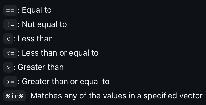
Here are the different comparisons you can use with the filter( ) command. These are called comparison operators.


Let’s create a simple data frame to demonstrate how the filter( ) function works. We will use the data.frame() function to create a data frame with two columns: id and value. The id column will contain the numbers 1 through 15, and the value column will contain the numbers 5, 2, 9, 4, 6, 3, 8, 1, 7, 10, 2, 6, 8, 3, and 5. We will then use the filter( ) function to filter the data frame based on different conditions.

# Sample data frame
data <- data.frame(
  id = 1:15,
  value = c(5, 2, 9, 4, 6, 3, 8, 1, 7, 10, 2, 6, 8, 3, 5)
)

data
   id value
1   1     5
2   2     2
3   3     9
4   4     4
5   5     6
6   6     3
7   7     8
8   8     1
9   9     7
10 10    10
11 11     2
12 12     6
13 13     8
14 14     3
15 15     5


Here is an example of how to use the filter( ) function to filter the data frame to include only rows where the value is equal to 5.

# Filter rows where value is equal to 5
filtered_data_1 <- filter(data, value == 5)

# Print out the results
filtered_data_1
  id value
1  1     5
2 15     5


Here are more examples :

# Filter rows where value is not equal to 5
filtered_data_2 <- filter(data, value != 5)

filtered_data_2
   id value
1   2     2
2   3     9
3   4     4
4   5     6
5   6     3
6   7     8
7   8     1
8   9     7
9  10    10
10 11     2
11 12     6
12 13     8
13 14     3
# Filter rows where value is less than 5
filtered_data_3 <- filter(data, value < 5)

filtered_data_3
  id value
1  2     2
2  4     4
3  6     3
4  8     1
5 11     2
6 14     3
# Filter rows where value is less than or equal to 3
filtered_data_4 <- filter(data, value <= 3)

filtered_data_4
  id value
1  2     2
2  6     3
3  8     1
4 11     2
5 14     3
# Filter rows where value is greater than 8
filtered_data_5 <- filter(data, value > 8)

filtered_data_5
  id value
1  3     9
2 10    10
# Filter rows where value is greater than or equal to 7
filtered_data_6 <- filter(data, value >= 7)

filtered_data_6
  id value
1  3     9
2  7     8
3  9     7
4 10    10
5 13     8
# Filter rows where value is in the set of 1, 5, or 10
filtered_data_7 <- filter(data, value %in% c(1, 5, 10))

filtered_data_7
  id value
1  1     5
2  8     1
3 10    10
4 15     5

Going back to the mtcars example, if you want to filter the data to include only rows where the number of cylinders is 6, you can use the following command:


# reinitialize the data set

data <- mtcars

# Filter the data to include only rows where the number of cylinders is 6

data %>%
  filter(cyl == 6)
                mpg cyl  disp  hp drat    wt  qsec vs am gear carb
Mazda RX4      21.0   6 160.0 110 3.90 2.620 16.46  0  1    4    4
Mazda RX4 Wag  21.0   6 160.0 110 3.90 2.875 17.02  0  1    4    4
Hornet 4 Drive 21.4   6 258.0 110 3.08 3.215 19.44  1  0    3    1
Valiant        18.1   6 225.0 105 2.76 3.460 20.22  1  0    3    1
Merc 280       19.2   6 167.6 123 3.92 3.440 18.30  1  0    4    4
Merc 280C      17.8   6 167.6 123 3.92 3.440 18.90  1  0    4    4
Ferrari Dino   19.7   6 145.0 175 3.62 2.770 15.50  0  1    5    6


As you can see from the output, the data has been filtered to include only rows where the number of cylinders is 6. This is a simple example, but you can use the filter() function to filter the data based on any condition.

You can also use the filter() function from the dplyr package in combination with the is.na( ) and !is.na( ) functions to filter rows based on whether they contain NA (missing) values or not.

Here are examples of how to use filter( ) with is.na( ) and !is.na( ):

# Create a sample data frame
data <- data.frame(
  id = 1:10,
  value = c(5, NA, 9, 4, NA, 3, 8, 1, NA, 10)
)

# Filter rows where the 'value' column has NA values
filtered_data_na <- filter(data, is.na(value))
print(filtered_data_na)
  id value
1  2    NA
2  5    NA
3  9    NA
# Filter rows where the 'value' column does not have NA values
filtered_data_not_na <- filter(data, !is.na(value))
print(filtered_data_not_na)
  id value
1  1     5
2  3     9
3  4     4
4  6     3
5  7     8
6  8     1
7 10    10


Lastly, we can use the filter() function to filter the data based on multiple conditions. You can specify multiple conditions by passing them as arguments to the filter() function. Here are the logical operators you can use to combine multiple conditions:


Recall that the AND operator means we want all of the conditions to be true. The OR operator means we want at least one of the conditions to be true. The NOT operator means we want the condition to be false.

We will use this data set for the next few examples.

# Create a sample data frame
data <- data.frame(
  id = 1:15,
  value = c(3, 5, 7, 2, 8, 9, 10, 1, 4, 6, 3, 8, 1, 7, 10),
  category = c("C", "A", "B", "C", "C", "A", "B", "C", "A", "B", "A", "C", "B", "A", "B")
)

data
   id value category
1   1     3        C
2   2     5        A
3   3     7        B
4   4     2        C
5   5     8        C
6   6     9        A
7   7    10        B
8   8     1        C
9   9     4        A
10 10     6        B
11 11     3        A
12 12     8        C
13 13     1        B
14 14     7        A
15 15    10        B


Let’s filter the data to include only rows where the value is greater than 5 AND the category is “A”.

# Filter rows where 'value' is greater than 5 AND 'category' is 'A'
filtered_data_and <- filter(data, value > 8 & category == "A")

filtered_data_and
  id value category
1  6     9        A

In this example, we only had one instance where the value was greater than 8 and the category was “A”. So, we only have one row in the output.

Next we will filter the data to include only rows where the value is greater than 5 OR the category is “B”.

# Filter rows where 'value' is greater than 5 OR 'category' is 'B'
filtered_data_or <- filter(data, value <= 2 | category == "B")

filtered_data_or
  id value category
1  3     7        B
2  4     2        C
3  7    10        B
4  8     1        C
5 10     6        B
6 13     1        B
7 15    10        B

This example gave us many more rows in the output because we are looking for rows where the value is less than or equal to 2 or the category is “B”. The OR command is less restrictive than the AND command, usually leading to more rows in the output.

Finally, we will filter the data to include only rows where the value is not equal to 5.

# Filter rows where 'value' is not equal to 5

filtered_data_not <- filter(data, value != 5)

filtered_data_not
   id value category
1   1     3        C
2   3     7        B
3   4     2        C
4   5     8        C
5   6     9        A
6   7    10        B
7   8     1        C
8   9     4        A
9  10     6        B
10 11     3        A
11 12     8        C
12 13     1        B
13 14     7        A
14 15    10        B

Here we have plenty of results where the value is not equal to 5.

mutate( )

When using the mutate() function, we can create new columns based on existing columns in the data set. You do have to be careful if you want to save the new data set with the new column. If you don’t assign the output to a new variable, the new column will not be saved.

Let’s use the mutate() function to create a new column called gpm that calculates the miles per gallon (mpg) per cylinder (cyl). This will give us a measure of fuel efficiency per cylinder.

# reinitialize the data set

data <- mtcars

# Create a new column called "gpm" that calculates the miles per gallon per cylinder

data %>%
  mutate(gpm = mpg / cyl)
                     mpg cyl  disp  hp drat    wt  qsec vs am gear carb
Mazda RX4           21.0   6 160.0 110 3.90 2.620 16.46  0  1    4    4
Mazda RX4 Wag       21.0   6 160.0 110 3.90 2.875 17.02  0  1    4    4
Datsun 710          22.8   4 108.0  93 3.85 2.320 18.61  1  1    4    1
Hornet 4 Drive      21.4   6 258.0 110 3.08 3.215 19.44  1  0    3    1
Hornet Sportabout   18.7   8 360.0 175 3.15 3.440 17.02  0  0    3    2
Valiant             18.1   6 225.0 105 2.76 3.460 20.22  1  0    3    1
Duster 360          14.3   8 360.0 245 3.21 3.570 15.84  0  0    3    4
Merc 240D           24.4   4 146.7  62 3.69 3.190 20.00  1  0    4    2
Merc 230            22.8   4 140.8  95 3.92 3.150 22.90  1  0    4    2
Merc 280            19.2   6 167.6 123 3.92 3.440 18.30  1  0    4    4
Merc 280C           17.8   6 167.6 123 3.92 3.440 18.90  1  0    4    4
Merc 450SE          16.4   8 275.8 180 3.07 4.070 17.40  0  0    3    3
Merc 450SL          17.3   8 275.8 180 3.07 3.730 17.60  0  0    3    3
Merc 450SLC         15.2   8 275.8 180 3.07 3.780 18.00  0  0    3    3
Cadillac Fleetwood  10.4   8 472.0 205 2.93 5.250 17.98  0  0    3    4
Lincoln Continental 10.4   8 460.0 215 3.00 5.424 17.82  0  0    3    4
Chrysler Imperial   14.7   8 440.0 230 3.23 5.345 17.42  0  0    3    4
Fiat 128            32.4   4  78.7  66 4.08 2.200 19.47  1  1    4    1
Honda Civic         30.4   4  75.7  52 4.93 1.615 18.52  1  1    4    2
Toyota Corolla      33.9   4  71.1  65 4.22 1.835 19.90  1  1    4    1
Toyota Corona       21.5   4 120.1  97 3.70 2.465 20.01  1  0    3    1
Dodge Challenger    15.5   8 318.0 150 2.76 3.520 16.87  0  0    3    2
AMC Javelin         15.2   8 304.0 150 3.15 3.435 17.30  0  0    3    2
Camaro Z28          13.3   8 350.0 245 3.73 3.840 15.41  0  0    3    4
Pontiac Firebird    19.2   8 400.0 175 3.08 3.845 17.05  0  0    3    2
Fiat X1-9           27.3   4  79.0  66 4.08 1.935 18.90  1  1    4    1
Porsche 914-2       26.0   4 120.3  91 4.43 2.140 16.70  0  1    5    2
Lotus Europa        30.4   4  95.1 113 3.77 1.513 16.90  1  1    5    2
Ford Pantera L      15.8   8 351.0 264 4.22 3.170 14.50  0  1    5    4
Ferrari Dino        19.7   6 145.0 175 3.62 2.770 15.50  0  1    5    6
Maserati Bora       15.0   8 301.0 335 3.54 3.570 14.60  0  1    5    8
Volvo 142E          21.4   4 121.0 109 4.11 2.780 18.60  1  1    4    2
                         gpm
Mazda RX4           3.500000
Mazda RX4 Wag       3.500000
Datsun 710          5.700000
Hornet 4 Drive      3.566667
Hornet Sportabout   2.337500
Valiant             3.016667
Duster 360          1.787500
Merc 240D           6.100000
Merc 230            5.700000
Merc 280            3.200000
Merc 280C           2.966667
Merc 450SE          2.050000
Merc 450SL          2.162500
Merc 450SLC         1.900000
Cadillac Fleetwood  1.300000
Lincoln Continental 1.300000
Chrysler Imperial   1.837500
Fiat 128            8.100000
Honda Civic         7.600000
Toyota Corolla      8.475000
Toyota Corona       5.375000
Dodge Challenger    1.937500
AMC Javelin         1.900000
Camaro Z28          1.662500
Pontiac Firebird    2.400000
Fiat X1-9           6.825000
Porsche 914-2       6.500000
Lotus Europa        7.600000
Ford Pantera L      1.975000
Ferrari Dino        3.283333
Maserati Bora       1.875000
Volvo 142E          5.350000

At this point we have not saved the new data set with the new column. If you look at the data set, you will see that the new column has not been saved.

head(data)
                   mpg cyl disp  hp drat    wt  qsec vs am gear carb
Mazda RX4         21.0   6  160 110 3.90 2.620 16.46  0  1    4    4
Mazda RX4 Wag     21.0   6  160 110 3.90 2.875 17.02  0  1    4    4
Datsun 710        22.8   4  108  93 3.85 2.320 18.61  1  1    4    1
Hornet 4 Drive    21.4   6  258 110 3.08 3.215 19.44  1  0    3    1
Hornet Sportabout 18.7   8  360 175 3.15 3.440 17.02  0  0    3    2
Valiant           18.1   6  225 105 2.76 3.460 20.22  1  0    3    1
# If we want to save the new data set with the new column, we need to assign the
# output to a new variable.

data2 <- data %>%
  mutate(gpm = mpg / cyl)

# Notice that the output did not get printed out. It was saved to the new
# variable data2. data2 is a new data set with the new column has been saved.

head(data2)
                   mpg cyl disp  hp drat    wt  qsec vs am gear carb      gpm
Mazda RX4         21.0   6  160 110 3.90 2.620 16.46  0  1    4    4 3.500000
Mazda RX4 Wag     21.0   6  160 110 3.90 2.875 17.02  0  1    4    4 3.500000
Datsun 710        22.8   4  108  93 3.85 2.320 18.61  1  1    4    1 5.700000
Hornet 4 Drive    21.4   6  258 110 3.08 3.215 19.44  1  0    3    1 3.566667
Hornet Sportabout 18.7   8  360 175 3.15 3.440 17.02  0  0    3    2 2.337500
Valiant           18.1   6  225 105 2.76 3.460 20.22  1  0    3    1 3.016667


We can now use data2 for further analysis or if we need the new column for any other purpose.

It is also possible to use the mutate() function to create multiple new columns at once. You can specify the new columns you want to create by passing them as arguments to the mutate() function. Let’s use the mutate() function to create two new columns: gpm (miles per gallon per cylinder) and hp_per_cyl (horsepower per cylinder).

# Create two new columns: "gpm" and "hp_per_cyl"

data %>%
  mutate(gpm = mpg / cyl,
         hp_per_cyl = hp / cyl)
                     mpg cyl  disp  hp drat    wt  qsec vs am gear carb
Mazda RX4           21.0   6 160.0 110 3.90 2.620 16.46  0  1    4    4
Mazda RX4 Wag       21.0   6 160.0 110 3.90 2.875 17.02  0  1    4    4
Datsun 710          22.8   4 108.0  93 3.85 2.320 18.61  1  1    4    1
Hornet 4 Drive      21.4   6 258.0 110 3.08 3.215 19.44  1  0    3    1
Hornet Sportabout   18.7   8 360.0 175 3.15 3.440 17.02  0  0    3    2
Valiant             18.1   6 225.0 105 2.76 3.460 20.22  1  0    3    1
Duster 360          14.3   8 360.0 245 3.21 3.570 15.84  0  0    3    4
Merc 240D           24.4   4 146.7  62 3.69 3.190 20.00  1  0    4    2
Merc 230            22.8   4 140.8  95 3.92 3.150 22.90  1  0    4    2
Merc 280            19.2   6 167.6 123 3.92 3.440 18.30  1  0    4    4
Merc 280C           17.8   6 167.6 123 3.92 3.440 18.90  1  0    4    4
Merc 450SE          16.4   8 275.8 180 3.07 4.070 17.40  0  0    3    3
Merc 450SL          17.3   8 275.8 180 3.07 3.730 17.60  0  0    3    3
Merc 450SLC         15.2   8 275.8 180 3.07 3.780 18.00  0  0    3    3
Cadillac Fleetwood  10.4   8 472.0 205 2.93 5.250 17.98  0  0    3    4
Lincoln Continental 10.4   8 460.0 215 3.00 5.424 17.82  0  0    3    4
Chrysler Imperial   14.7   8 440.0 230 3.23 5.345 17.42  0  0    3    4
Fiat 128            32.4   4  78.7  66 4.08 2.200 19.47  1  1    4    1
Honda Civic         30.4   4  75.7  52 4.93 1.615 18.52  1  1    4    2
Toyota Corolla      33.9   4  71.1  65 4.22 1.835 19.90  1  1    4    1
Toyota Corona       21.5   4 120.1  97 3.70 2.465 20.01  1  0    3    1
Dodge Challenger    15.5   8 318.0 150 2.76 3.520 16.87  0  0    3    2
AMC Javelin         15.2   8 304.0 150 3.15 3.435 17.30  0  0    3    2
Camaro Z28          13.3   8 350.0 245 3.73 3.840 15.41  0  0    3    4
Pontiac Firebird    19.2   8 400.0 175 3.08 3.845 17.05  0  0    3    2
Fiat X1-9           27.3   4  79.0  66 4.08 1.935 18.90  1  1    4    1
Porsche 914-2       26.0   4 120.3  91 4.43 2.140 16.70  0  1    5    2
Lotus Europa        30.4   4  95.1 113 3.77 1.513 16.90  1  1    5    2
Ford Pantera L      15.8   8 351.0 264 4.22 3.170 14.50  0  1    5    4
Ferrari Dino        19.7   6 145.0 175 3.62 2.770 15.50  0  1    5    6
Maserati Bora       15.0   8 301.0 335 3.54 3.570 14.60  0  1    5    8
Volvo 142E          21.4   4 121.0 109 4.11 2.780 18.60  1  1    4    2
                         gpm hp_per_cyl
Mazda RX4           3.500000   18.33333
Mazda RX4 Wag       3.500000   18.33333
Datsun 710          5.700000   23.25000
Hornet 4 Drive      3.566667   18.33333
Hornet Sportabout   2.337500   21.87500
Valiant             3.016667   17.50000
Duster 360          1.787500   30.62500
Merc 240D           6.100000   15.50000
Merc 230            5.700000   23.75000
Merc 280            3.200000   20.50000
Merc 280C           2.966667   20.50000
Merc 450SE          2.050000   22.50000
Merc 450SL          2.162500   22.50000
Merc 450SLC         1.900000   22.50000
Cadillac Fleetwood  1.300000   25.62500
Lincoln Continental 1.300000   26.87500
Chrysler Imperial   1.837500   28.75000
Fiat 128            8.100000   16.50000
Honda Civic         7.600000   13.00000
Toyota Corolla      8.475000   16.25000
Toyota Corona       5.375000   24.25000
Dodge Challenger    1.937500   18.75000
AMC Javelin         1.900000   18.75000
Camaro Z28          1.662500   30.62500
Pontiac Firebird    2.400000   21.87500
Fiat X1-9           6.825000   16.50000
Porsche 914-2       6.500000   22.75000
Lotus Europa        7.600000   28.25000
Ford Pantera L      1.975000   33.00000
Ferrari Dino        3.283333   29.16667
Maserati Bora       1.875000   41.87500
Volvo 142E          5.350000   27.25000

Don’t forget to save these new columns if you want to use them later on :

# Save the new data set with the new columns

data3 <- data %>%
  mutate(gpm = mpg / cyl,
         hp_per_cyl = hp / cyl)

head(data3)
                   mpg cyl disp  hp drat    wt  qsec vs am gear carb      gpm
Mazda RX4         21.0   6  160 110 3.90 2.620 16.46  0  1    4    4 3.500000
Mazda RX4 Wag     21.0   6  160 110 3.90 2.875 17.02  0  1    4    4 3.500000
Datsun 710        22.8   4  108  93 3.85 2.320 18.61  1  1    4    1 5.700000
Hornet 4 Drive    21.4   6  258 110 3.08 3.215 19.44  1  0    3    1 3.566667
Hornet Sportabout 18.7   8  360 175 3.15 3.440 17.02  0  0    3    2 2.337500
Valiant           18.1   6  225 105 2.76 3.460 20.22  1  0    3    1 3.016667
                  hp_per_cyl
Mazda RX4           18.33333
Mazda RX4 Wag       18.33333
Datsun 710          23.25000
Hornet 4 Drive      18.33333
Hornet Sportabout   21.87500
Valiant             17.50000


If needed, we can also use mutate() to change the values in an existing column. For example, if we wanted to add 1 to the cyl variable, we could use the following command:

# Original data set :

head(data)
                   mpg cyl disp  hp drat    wt  qsec vs am gear carb
Mazda RX4         21.0   6  160 110 3.90 2.620 16.46  0  1    4    4
Mazda RX4 Wag     21.0   6  160 110 3.90 2.875 17.02  0  1    4    4
Datsun 710        22.8   4  108  93 3.85 2.320 18.61  1  1    4    1
Hornet 4 Drive    21.4   6  258 110 3.08 3.215 19.44  1  0    3    1
Hornet Sportabout 18.7   8  360 175 3.15 3.440 17.02  0  0    3    2
Valiant           18.1   6  225 105 2.76 3.460 20.22  1  0    3    1
# Convert the miles per gallon (mpg) column to kilometers per liter (kpl)
  
data <- data %>%
  mutate(cyl = cyl + 1)
# New data set:

head(data)
                   mpg cyl disp  hp drat    wt  qsec vs am gear carb
Mazda RX4         21.0   7  160 110 3.90 2.620 16.46  0  1    4    4
Mazda RX4 Wag     21.0   7  160 110 3.90 2.875 17.02  0  1    4    4
Datsun 710        22.8   5  108  93 3.85 2.320 18.61  1  1    4    1
Hornet 4 Drive    21.4   7  258 110 3.08 3.215 19.44  1  0    3    1
Hornet Sportabout 18.7   9  360 175 3.15 3.440 17.02  0  0    3    2
Valiant           18.1   7  225 105 2.76 3.460 20.22  1  0    3    1

select( )

The select() function is used to select columns from the data set. You can specify the columns you want to keep by passing their names as arguments to the select() function. You can also use the : operator to select a range of columns. Let’s use the select() function to select the columns mpg, cyl, and hp from the data set.

# reinitialize the data set

data <- mtcars

# Select the columns mpg, cyl, and hp

data %>%
  select(mpg, cyl, hp)
                     mpg cyl  hp
Mazda RX4           21.0   6 110
Mazda RX4 Wag       21.0   6 110
Datsun 710          22.8   4  93
Hornet 4 Drive      21.4   6 110
Hornet Sportabout   18.7   8 175
Valiant             18.1   6 105
Duster 360          14.3   8 245
Merc 240D           24.4   4  62
Merc 230            22.8   4  95
Merc 280            19.2   6 123
Merc 280C           17.8   6 123
Merc 450SE          16.4   8 180
Merc 450SL          17.3   8 180
Merc 450SLC         15.2   8 180
Cadillac Fleetwood  10.4   8 205
Lincoln Continental 10.4   8 215
Chrysler Imperial   14.7   8 230
Fiat 128            32.4   4  66
Honda Civic         30.4   4  52
Toyota Corolla      33.9   4  65
Toyota Corona       21.5   4  97
Dodge Challenger    15.5   8 150
AMC Javelin         15.2   8 150
Camaro Z28          13.3   8 245
Pontiac Firebird    19.2   8 175
Fiat X1-9           27.3   4  66
Porsche 914-2       26.0   4  91
Lotus Europa        30.4   4 113
Ford Pantera L      15.8   8 264
Ferrari Dino        19.7   6 175
Maserati Bora       15.0   8 335
Volvo 142E          21.4   4 109


As you can see from the output, the data set has been filtered to include only the columns mpg, cyl, and hp. You can use the select() function to select any columns you want from the data set.

It is also worth noting that we did not save the new data set with the selected columns. If you want to save the new data set with the selected columns, you need to assign the output to a new variable.

# Save the new data set with the selected columns

data3 <- data %>%
  select(mpg, cyl, hp)

# Notice that the output did not get printed out. It was saved to the new
# variable data3. data3 is a new data set with the selected columns.

head(data3)
                   mpg cyl  hp
Mazda RX4         21.0   6 110
Mazda RX4 Wag     21.0   6 110
Datsun 710        22.8   4  93
Hornet 4 Drive    21.4   6 110
Hornet Sportabout 18.7   8 175
Valiant           18.1   6 105

We could also use the : operator to select a range of columns. For example, if we wanted to select all columns from mpg to hp, we could use the following command:

# Select all columns from mpg to hp and save the new data set to data4

data4 <- data %>%
  select(mpg:hp)

head(data4)
                   mpg cyl disp  hp
Mazda RX4         21.0   6  160 110
Mazda RX4 Wag     21.0   6  160 110
Datsun 710        22.8   4  108  93
Hornet 4 Drive    21.4   6  258 110
Hornet Sportabout 18.7   8  360 175
Valiant           18.1   6  225 105


If we want to exclude a column, we can use the - operator. For example, if we wanted to select all columns except mpg, we could use the following command:

# Select all columns except mpg and save the new data set to data5

data5 <- data %>%
  select(-mpg)

head(data5)
                  cyl disp  hp drat    wt  qsec vs am gear carb
Mazda RX4           6  160 110 3.90 2.620 16.46  0  1    4    4
Mazda RX4 Wag       6  160 110 3.90 2.875 17.02  0  1    4    4
Datsun 710          4  108  93 3.85 2.320 18.61  1  1    4    1
Hornet 4 Drive      6  258 110 3.08 3.215 19.44  1  0    3    1
Hornet Sportabout   8  360 175 3.15 3.440 17.02  0  0    3    2
Valiant             6  225 105 2.76 3.460 20.22  1  0    3    1

If we want to remove a range of columns, we can combine the last two ideas. For instance, if we want to remove the columns from mpg to hp, we could use the following command:

# Remove all columns from mpg to hp and save the new data set to data6

data6 <- data %>%
  select(-(mpg:hp))

head(data6)
                  drat    wt  qsec vs am gear carb
Mazda RX4         3.90 2.620 16.46  0  1    4    4
Mazda RX4 Wag     3.90 2.875 17.02  0  1    4    4
Datsun 710        3.85 2.320 18.61  1  1    4    1
Hornet 4 Drive    3.08 3.215 19.44  1  0    3    1
Hornet Sportabout 3.15 3.440 17.02  0  0    3    2
Valiant           2.76 3.460 20.22  1  0    3    1


arrange( )

The arrange() function is used to sort the data set based on one or more columns. You can specify the columns you want to sort by passing their names as arguments to the arrange() function. By default, the data set is sorted in ascending order. If you want to sort in descending order, you can use the desc() function. Let’s use the arrange() function to sort the data set by the mpg column in descending order.

# reinitialize the data set

data <- mtcars

# Sort the data set by the mpg column in descending order

data %>%
  arrange(desc(mpg))
                     mpg cyl  disp  hp drat    wt  qsec vs am gear carb
Toyota Corolla      33.9   4  71.1  65 4.22 1.835 19.90  1  1    4    1
Fiat 128            32.4   4  78.7  66 4.08 2.200 19.47  1  1    4    1
Honda Civic         30.4   4  75.7  52 4.93 1.615 18.52  1  1    4    2
Lotus Europa        30.4   4  95.1 113 3.77 1.513 16.90  1  1    5    2
Fiat X1-9           27.3   4  79.0  66 4.08 1.935 18.90  1  1    4    1
Porsche 914-2       26.0   4 120.3  91 4.43 2.140 16.70  0  1    5    2
Merc 240D           24.4   4 146.7  62 3.69 3.190 20.00  1  0    4    2
Datsun 710          22.8   4 108.0  93 3.85 2.320 18.61  1  1    4    1
Merc 230            22.8   4 140.8  95 3.92 3.150 22.90  1  0    4    2
Toyota Corona       21.5   4 120.1  97 3.70 2.465 20.01  1  0    3    1
Hornet 4 Drive      21.4   6 258.0 110 3.08 3.215 19.44  1  0    3    1
Volvo 142E          21.4   4 121.0 109 4.11 2.780 18.60  1  1    4    2
Mazda RX4           21.0   6 160.0 110 3.90 2.620 16.46  0  1    4    4
Mazda RX4 Wag       21.0   6 160.0 110 3.90 2.875 17.02  0  1    4    4
Ferrari Dino        19.7   6 145.0 175 3.62 2.770 15.50  0  1    5    6
Merc 280            19.2   6 167.6 123 3.92 3.440 18.30  1  0    4    4
Pontiac Firebird    19.2   8 400.0 175 3.08 3.845 17.05  0  0    3    2
Hornet Sportabout   18.7   8 360.0 175 3.15 3.440 17.02  0  0    3    2
Valiant             18.1   6 225.0 105 2.76 3.460 20.22  1  0    3    1
Merc 280C           17.8   6 167.6 123 3.92 3.440 18.90  1  0    4    4
Merc 450SL          17.3   8 275.8 180 3.07 3.730 17.60  0  0    3    3
Merc 450SE          16.4   8 275.8 180 3.07 4.070 17.40  0  0    3    3
Ford Pantera L      15.8   8 351.0 264 4.22 3.170 14.50  0  1    5    4
Dodge Challenger    15.5   8 318.0 150 2.76 3.520 16.87  0  0    3    2
Merc 450SLC         15.2   8 275.8 180 3.07 3.780 18.00  0  0    3    3
AMC Javelin         15.2   8 304.0 150 3.15 3.435 17.30  0  0    3    2
Maserati Bora       15.0   8 301.0 335 3.54 3.570 14.60  0  1    5    8
Chrysler Imperial   14.7   8 440.0 230 3.23 5.345 17.42  0  0    3    4
Duster 360          14.3   8 360.0 245 3.21 3.570 15.84  0  0    3    4
Camaro Z28          13.3   8 350.0 245 3.73 3.840 15.41  0  0    3    4
Cadillac Fleetwood  10.4   8 472.0 205 2.93 5.250 17.98  0  0    3    4
Lincoln Continental 10.4   8 460.0 215 3.00 5.424 17.82  0  0    3    4


As we saw above, the output is not saved. If you want to save the sorted data set, you need to assign the output to a new variable.

# Save the sorted data set to data6

data6 <- data %>%
  arrange(desc(mpg))

head(data6)
                mpg cyl  disp  hp drat    wt  qsec vs am gear carb
Toyota Corolla 33.9   4  71.1  65 4.22 1.835 19.90  1  1    4    1
Fiat 128       32.4   4  78.7  66 4.08 2.200 19.47  1  1    4    1
Honda Civic    30.4   4  75.7  52 4.93 1.615 18.52  1  1    4    2
Lotus Europa   30.4   4  95.1 113 3.77 1.513 16.90  1  1    5    2
Fiat X1-9      27.3   4  79.0  66 4.08 1.935 18.90  1  1    4    1
Porsche 914-2  26.0   4 120.3  91 4.43 2.140 16.70  0  1    5    2


We can sort the data set by multiple columns by passing multiple arguments to the arrange() function. For example, if we wanted to sort the data set by the mpg column in descending order and then by the cyl column in ascending order, we could use the following command:

# Sort the data set by the mpg column in descending order and then by the cyl 
# column in ascending order and save the output to data7

data7 <- data %>%
  arrange(desc(mpg), cyl)

head(data7)
                mpg cyl  disp  hp drat    wt  qsec vs am gear carb
Toyota Corolla 33.9   4  71.1  65 4.22 1.835 19.90  1  1    4    1
Fiat 128       32.4   4  78.7  66 4.08 2.200 19.47  1  1    4    1
Honda Civic    30.4   4  75.7  52 4.93 1.615 18.52  1  1    4    2
Lotus Europa   30.4   4  95.1 113 3.77 1.513 16.90  1  1    5    2
Fiat X1-9      27.3   4  79.0  66 4.08 1.935 18.90  1  1    4    1
Porsche 914-2  26.0   4 120.3  91 4.43 2.140 16.70  0  1    5    2
tail(data7)
                     mpg cyl disp  hp drat    wt  qsec vs am gear carb
Maserati Bora       15.0   8  301 335 3.54 3.570 14.60  0  1    5    8
Chrysler Imperial   14.7   8  440 230 3.23 5.345 17.42  0  0    3    4
Duster 360          14.3   8  360 245 3.21 3.570 15.84  0  0    3    4
Camaro Z28          13.3   8  350 245 3.73 3.840 15.41  0  0    3    4
Cadillac Fleetwood  10.4   8  472 205 2.93 5.250 17.98  0  0    3    4
Lincoln Continental 10.4   8  460 215 3.00 5.424 17.82  0  0    3    4


You can see from the head( ) and tail( ) commands that the data set has been sorted first by the mpg column in descending order and then by the cyl column in ascending order. So the cars with 4 cylinders come first and they are sorted by the miles per gallon in descending order. Then the cars with 6 cylinders come next and they are also sorted by the miles per gallon in descending order. Finally, the cars with 8 cylinders come last and they are also sorted by the miles per gallon in descending order.

group_by( ) and summarize( )

The group_by() function is used to group the data set by one or more columns. The summarize() function is used to summarize the data within each group. You can specify the summary statistics you want to calculate by passing them as arguments to the summarize() function. Let’s use the group_by() and summarize() functions to calculate the average miles per gallon (mpg) for each number of cylinders (cyl).

# reinitialize the data set

data <- mtcars

# Group the data set by the cyl column and calculate the average mpg for each group

data %>%
  group_by(cyl) %>%
  summarize(avg_mpg = mean(mpg))
# A tibble: 3 × 2
    cyl avg_mpg
  <dbl>   <dbl>
1     4    26.7
2     6    19.7
3     8    15.1


In this example, the data was grouped together by cylinders and then the average was calculated to the miles per gallon for each group.

Let’s verify this result by looking at the cars with 6 cylinders. Let us filter the data set to include only cars with 6 cylinders and then calculate the average miles per gallon for these cars.

# Filter the data set to include only cars with 6 cylinders

cyl6_data <- data %>%
  filter(cyl == 6)

cyl6_data
                mpg cyl  disp  hp drat    wt  qsec vs am gear carb
Mazda RX4      21.0   6 160.0 110 3.90 2.620 16.46  0  1    4    4
Mazda RX4 Wag  21.0   6 160.0 110 3.90 2.875 17.02  0  1    4    4
Hornet 4 Drive 21.4   6 258.0 110 3.08 3.215 19.44  1  0    3    1
Valiant        18.1   6 225.0 105 2.76 3.460 20.22  1  0    3    1
Merc 280       19.2   6 167.6 123 3.92 3.440 18.30  1  0    4    4
Merc 280C      17.8   6 167.6 123 3.92 3.440 18.90  1  0    4    4
Ferrari Dino   19.7   6 145.0 175 3.62 2.770 15.50  0  1    5    6


We can now calculate the average miles per gallon for these cars.

# Calculate the average miles per gallon for cars with 6 cylinders

mean(cyl6_data$mpg)
[1] 19.74286


Tip

As you are coding, it is always good to double check your work with a small subset of the data to make sure that you are getting the results you expect.

As we saw above, the output is not saved as we are just printing out the result. If you want to save the summarized data set, you need to assign the output to a new variable.

# Save the summarized data set to data8

data8 <- data %>%
  group_by(cyl) %>%
  summarize(avg_mpg = mean(mpg))

data8
# A tibble: 3 × 2
    cyl avg_mpg
  <dbl>   <dbl>
1     4    26.7
2     6    19.7
3     8    15.1


What happens if we have data that is incomplete? In other words, what if we have missing values in our data set? Let’s take a look at the airquality data set, which contains information about air quality measurements in New York City. This data set has missing values, so we need to be careful when calculating summary statistics.

# Load the airquality data set

data("airquality")

# Print out the first few rows of the data set

head(airquality)
  Ozone Solar.R Wind Temp Month Day
1    41     190  7.4   67     5   1
2    36     118  8.0   72     5   2
3    12     149 12.6   74     5   3
4    18     313 11.5   62     5   4
5    NA      NA 14.3   56     5   5
6    28      NA 14.9   66     5   6

Let’s calculate the average Solar.R value for each month in the airquality data set. We will use the group_by() and summarize() functions to group the data by the Month column and calculate the average temperature for each month.

# Group the data set by the Month column and calculate the average Temp for each group

airquality %>%
  group_by(Month) %>%
  summarize(avg_temp = mean(Solar.R))
# A tibble: 5 × 2
  Month avg_temp
  <int>    <dbl>
1     5      NA 
2     6     190.
3     7     216.
4     8      NA 
5     9     167.

You can see that the NA values did not allow us to properly calculate the mean. R does not automatically drop the NA vaules when going through the calculations. We can use the na.rm = TRUE argument to remove the NA values and calculate the mean for the remaining values.

# Group the data set by the Month column and calculate the average Solar.R for each group

airquality %>%
  group_by(Month) %>%
  summarize(avg_temp = mean(Solar.R, na.rm = TRUE))
# A tibble: 5 × 2
  Month avg_temp
  <int>    <dbl>
1     5     181.
2     6     190.
3     7     216.
4     8     172.
5     9     167.

There are many other functions that you can use with summarize() other than just mean(). Here are some of the other functions that you can use:

  • mean(): Calculate the mean
  • median(): Calculate the median
  • sd(): Calculate the standard deviation
  • var(): Calculate the variance
  • min(): Calculate the minimum value
  • max(): Calculate the maximum value
  • n(): Count the number of observations
  • sum(): Calculate the sum
  • first(): Get the first value
  • last(): Get the last value
  • nth(): Get the nth value
  • n_distinct(): Count the number of distinct values

You can use these functions to calculate a wide range of summary statistics for your data.

Here is an example of how to use the summarize() function to find the number of unique values in the Month column of the airquality data set.

# Find the number of unique values in the Month column

airquality %>%
  summarize(unique_months = n_distinct(Month))
  unique_months
1             5

Chaining Operations

One of the powerful features of the dplyr package is the ability to chain operations together using the piping operator %>%. This allows you to perform multiple data manipulation steps in a single line of code. Let’s walk through an example to see how this works.

Suppose we want to filter the mtcars data set to include only cars with 6 cylinders, select the mpg, cyl, and hp columns, and then arrange the data by the mpg column in descending order. We can do this in a single line of code using the piping operator %>%.

# reinitialize the data set

data <- mtcars

# Filter the data to include only cars with 6 cylinders, select the mpg, cyl, 
# and hp columns, and arrange the data by the mpg column in descending order

data %>%
  filter(cyl == 6) %>%
  select(mpg, cyl, hp) %>%
  arrange(desc(mpg))
                mpg cyl  hp
Hornet 4 Drive 21.4   6 110
Mazda RX4      21.0   6 110
Mazda RX4 Wag  21.0   6 110
Ferrari Dino   19.7   6 175
Merc 280       19.2   6 123
Valiant        18.1   6 105
Merc 280C      17.8   6 123

Another example is to filter the mtcars data set to include only cars with 6 cylinders, create a new column power_to_weight that calculates the ratio of hp to wt, and then select the mpg, cyl, hp, and power_to_weight columns.

# reinitialize the data set

data <- mtcars

# Filter the data to include only cars with 6 cylinders, create a new column
# power_to_weight that calculates the ratio of hp to wt, and select the mpg, cyl,
# hp, and power_to_weight columns

data %>%
  filter(cyl == 6) %>%
  mutate(power_to_weight = hp / wt) %>%
  select(mpg, cyl, hp, power_to_weight)
                mpg cyl  hp power_to_weight
Mazda RX4      21.0   6 110        41.98473
Mazda RX4 Wag  21.0   6 110        38.26087
Hornet 4 Drive 21.4   6 110        34.21462
Valiant        18.1   6 105        30.34682
Merc 280       19.2   6 123        35.75581
Merc 280C      17.8   6 123        35.75581
Ferrari Dino   19.7   6 175        63.17690


Conclusion

In this tutorial, we learned how to clean data using the dplyr package. We saw several of the key functions in dplyr, including filter(), mutate(), select(), arrange(), group_by(), and summarize(). We also learned how to chain operations together using the piping operator %>%. These functions are powerful tools for data manipulation in R and can help you clean and transform your data quickly and efficiently.

For more information on the dplyr package, check out the documentation at https://dplyr.tidyverse.org/.


Practice Problems

Instructions: Solve each of the following problems using the commands we saw earlier from the dplyr package :

  • chaining operations with the %>% (piping) operator
  • filter(): Filter rows based on conditions
  • mutate(): Create new columns
  • select(): Select columns
  • arrange(): Arrange rows
  • group_by(): Group data
  • summarize(): Summarize data

Each of the solutions should be one piped command. Some may be a single pipe while others may take multiple pipes.

Problem 1: Filtering Rows

Use the mtcars dataset to filter the rows where the mpg (miles per gallon) is greater than 20. Save the result to filtered_mtcars.

Code
# Solution

# Check to see if your output matches the solution

# If needed, load up dplyr

# library(dplyr)

filtered_mtcars <- mtcars %>%
  filter(mpg > 20)

filtered_mtcars
                mpg cyl  disp  hp drat    wt  qsec vs am gear carb
Mazda RX4      21.0   6 160.0 110 3.90 2.620 16.46  0  1    4    4
Mazda RX4 Wag  21.0   6 160.0 110 3.90 2.875 17.02  0  1    4    4
Datsun 710     22.8   4 108.0  93 3.85 2.320 18.61  1  1    4    1
Hornet 4 Drive 21.4   6 258.0 110 3.08 3.215 19.44  1  0    3    1
Merc 240D      24.4   4 146.7  62 3.69 3.190 20.00  1  0    4    2
Merc 230       22.8   4 140.8  95 3.92 3.150 22.90  1  0    4    2
Fiat 128       32.4   4  78.7  66 4.08 2.200 19.47  1  1    4    1
Honda Civic    30.4   4  75.7  52 4.93 1.615 18.52  1  1    4    2
Toyota Corolla 33.9   4  71.1  65 4.22 1.835 19.90  1  1    4    1
Toyota Corona  21.5   4 120.1  97 3.70 2.465 20.01  1  0    3    1
Fiat X1-9      27.3   4  79.0  66 4.08 1.935 18.90  1  1    4    1
Porsche 914-2  26.0   4 120.3  91 4.43 2.140 16.70  0  1    5    2
Lotus Europa   30.4   4  95.1 113 3.77 1.513 16.90  1  1    5    2
Volvo 142E     21.4   4 121.0 109 4.11 2.780 18.60  1  1    4    2

Problem 2: Selecting Columns

Use the mtcars dataset to select the columns mpg, cyl, and hp. Save the result to selected_mtcars.

Code
# Solution

selected_mtcars <- mtcars %>%
  select(mpg, cyl, hp)

selected_mtcars
                     mpg cyl  hp
Mazda RX4           21.0   6 110
Mazda RX4 Wag       21.0   6 110
Datsun 710          22.8   4  93
Hornet 4 Drive      21.4   6 110
Hornet Sportabout   18.7   8 175
Valiant             18.1   6 105
Duster 360          14.3   8 245
Merc 240D           24.4   4  62
Merc 230            22.8   4  95
Merc 280            19.2   6 123
Merc 280C           17.8   6 123
Merc 450SE          16.4   8 180
Merc 450SL          17.3   8 180
Merc 450SLC         15.2   8 180
Cadillac Fleetwood  10.4   8 205
Lincoln Continental 10.4   8 215
Chrysler Imperial   14.7   8 230
Fiat 128            32.4   4  66
Honda Civic         30.4   4  52
Toyota Corolla      33.9   4  65
Toyota Corona       21.5   4  97
Dodge Challenger    15.5   8 150
AMC Javelin         15.2   8 150
Camaro Z28          13.3   8 245
Pontiac Firebird    19.2   8 175
Fiat X1-9           27.3   4  66
Porsche 914-2       26.0   4  91
Lotus Europa        30.4   4 113
Ford Pantera L      15.8   8 264
Ferrari Dino        19.7   6 175
Maserati Bora       15.0   8 335
Volvo 142E          21.4   4 109

Problem 3: Arranging Rows

Use the mtcars dataset to arrange the rows in descending order of hp (horsepower). Save the result to arranged_mtcars.

Code
# Solution

arranged_mtcars <- mtcars %>%
  arrange(desc(hp))

arranged_mtcars
                     mpg cyl  disp  hp drat    wt  qsec vs am gear carb
Maserati Bora       15.0   8 301.0 335 3.54 3.570 14.60  0  1    5    8
Ford Pantera L      15.8   8 351.0 264 4.22 3.170 14.50  0  1    5    4
Duster 360          14.3   8 360.0 245 3.21 3.570 15.84  0  0    3    4
Camaro Z28          13.3   8 350.0 245 3.73 3.840 15.41  0  0    3    4
Chrysler Imperial   14.7   8 440.0 230 3.23 5.345 17.42  0  0    3    4
Lincoln Continental 10.4   8 460.0 215 3.00 5.424 17.82  0  0    3    4
Cadillac Fleetwood  10.4   8 472.0 205 2.93 5.250 17.98  0  0    3    4
Merc 450SE          16.4   8 275.8 180 3.07 4.070 17.40  0  0    3    3
Merc 450SL          17.3   8 275.8 180 3.07 3.730 17.60  0  0    3    3
Merc 450SLC         15.2   8 275.8 180 3.07 3.780 18.00  0  0    3    3
Hornet Sportabout   18.7   8 360.0 175 3.15 3.440 17.02  0  0    3    2
Pontiac Firebird    19.2   8 400.0 175 3.08 3.845 17.05  0  0    3    2
Ferrari Dino        19.7   6 145.0 175 3.62 2.770 15.50  0  1    5    6
Dodge Challenger    15.5   8 318.0 150 2.76 3.520 16.87  0  0    3    2
AMC Javelin         15.2   8 304.0 150 3.15 3.435 17.30  0  0    3    2
Merc 280            19.2   6 167.6 123 3.92 3.440 18.30  1  0    4    4
Merc 280C           17.8   6 167.6 123 3.92 3.440 18.90  1  0    4    4
Lotus Europa        30.4   4  95.1 113 3.77 1.513 16.90  1  1    5    2
Mazda RX4           21.0   6 160.0 110 3.90 2.620 16.46  0  1    4    4
Mazda RX4 Wag       21.0   6 160.0 110 3.90 2.875 17.02  0  1    4    4
Hornet 4 Drive      21.4   6 258.0 110 3.08 3.215 19.44  1  0    3    1
Volvo 142E          21.4   4 121.0 109 4.11 2.780 18.60  1  1    4    2
Valiant             18.1   6 225.0 105 2.76 3.460 20.22  1  0    3    1
Toyota Corona       21.5   4 120.1  97 3.70 2.465 20.01  1  0    3    1
Merc 230            22.8   4 140.8  95 3.92 3.150 22.90  1  0    4    2
Datsun 710          22.8   4 108.0  93 3.85 2.320 18.61  1  1    4    1
Porsche 914-2       26.0   4 120.3  91 4.43 2.140 16.70  0  1    5    2
Fiat 128            32.4   4  78.7  66 4.08 2.200 19.47  1  1    4    1
Fiat X1-9           27.3   4  79.0  66 4.08 1.935 18.90  1  1    4    1
Toyota Corolla      33.9   4  71.1  65 4.22 1.835 19.90  1  1    4    1
Merc 240D           24.4   4 146.7  62 3.69 3.190 20.00  1  0    4    2
Honda Civic         30.4   4  75.7  52 4.93 1.615 18.52  1  1    4    2

Problem 4: Creating New Columns

Use the mtcars dataset to create a new column power_to_weight which is the ratio of hp (horsepower) to wt (weight). Save the result to mutated_mtcars.

Code
# Solution

mutated_mtcars <- mtcars %>%
  mutate(power_to_weight = hp / wt)

mutated_mtcars
                     mpg cyl  disp  hp drat    wt  qsec vs am gear carb
Mazda RX4           21.0   6 160.0 110 3.90 2.620 16.46  0  1    4    4
Mazda RX4 Wag       21.0   6 160.0 110 3.90 2.875 17.02  0  1    4    4
Datsun 710          22.8   4 108.0  93 3.85 2.320 18.61  1  1    4    1
Hornet 4 Drive      21.4   6 258.0 110 3.08 3.215 19.44  1  0    3    1
Hornet Sportabout   18.7   8 360.0 175 3.15 3.440 17.02  0  0    3    2
Valiant             18.1   6 225.0 105 2.76 3.460 20.22  1  0    3    1
Duster 360          14.3   8 360.0 245 3.21 3.570 15.84  0  0    3    4
Merc 240D           24.4   4 146.7  62 3.69 3.190 20.00  1  0    4    2
Merc 230            22.8   4 140.8  95 3.92 3.150 22.90  1  0    4    2
Merc 280            19.2   6 167.6 123 3.92 3.440 18.30  1  0    4    4
Merc 280C           17.8   6 167.6 123 3.92 3.440 18.90  1  0    4    4
Merc 450SE          16.4   8 275.8 180 3.07 4.070 17.40  0  0    3    3
Merc 450SL          17.3   8 275.8 180 3.07 3.730 17.60  0  0    3    3
Merc 450SLC         15.2   8 275.8 180 3.07 3.780 18.00  0  0    3    3
Cadillac Fleetwood  10.4   8 472.0 205 2.93 5.250 17.98  0  0    3    4
Lincoln Continental 10.4   8 460.0 215 3.00 5.424 17.82  0  0    3    4
Chrysler Imperial   14.7   8 440.0 230 3.23 5.345 17.42  0  0    3    4
Fiat 128            32.4   4  78.7  66 4.08 2.200 19.47  1  1    4    1
Honda Civic         30.4   4  75.7  52 4.93 1.615 18.52  1  1    4    2
Toyota Corolla      33.9   4  71.1  65 4.22 1.835 19.90  1  1    4    1
Toyota Corona       21.5   4 120.1  97 3.70 2.465 20.01  1  0    3    1
Dodge Challenger    15.5   8 318.0 150 2.76 3.520 16.87  0  0    3    2
AMC Javelin         15.2   8 304.0 150 3.15 3.435 17.30  0  0    3    2
Camaro Z28          13.3   8 350.0 245 3.73 3.840 15.41  0  0    3    4
Pontiac Firebird    19.2   8 400.0 175 3.08 3.845 17.05  0  0    3    2
Fiat X1-9           27.3   4  79.0  66 4.08 1.935 18.90  1  1    4    1
Porsche 914-2       26.0   4 120.3  91 4.43 2.140 16.70  0  1    5    2
Lotus Europa        30.4   4  95.1 113 3.77 1.513 16.90  1  1    5    2
Ford Pantera L      15.8   8 351.0 264 4.22 3.170 14.50  0  1    5    4
Ferrari Dino        19.7   6 145.0 175 3.62 2.770 15.50  0  1    5    6
Maserati Bora       15.0   8 301.0 335 3.54 3.570 14.60  0  1    5    8
Volvo 142E          21.4   4 121.0 109 4.11 2.780 18.60  1  1    4    2
                    power_to_weight
Mazda RX4                  41.98473
Mazda RX4 Wag              38.26087
Datsun 710                 40.08621
Hornet 4 Drive             34.21462
Hornet Sportabout          50.87209
Valiant                    30.34682
Duster 360                 68.62745
Merc 240D                  19.43574
Merc 230                   30.15873
Merc 280                   35.75581
Merc 280C                  35.75581
Merc 450SE                 44.22604
Merc 450SL                 48.25737
Merc 450SLC                47.61905
Cadillac Fleetwood         39.04762
Lincoln Continental        39.63864
Chrysler Imperial          43.03087
Fiat 128                   30.00000
Honda Civic                32.19814
Toyota Corolla             35.42234
Toyota Corona              39.35091
Dodge Challenger           42.61364
AMC Javelin                43.66812
Camaro Z28                 63.80208
Pontiac Firebird           45.51365
Fiat X1-9                  34.10853
Porsche 914-2              42.52336
Lotus Europa               74.68605
Ford Pantera L             83.28076
Ferrari Dino               63.17690
Maserati Bora              93.83754
Volvo 142E                 39.20863

Problem 5: Summarizing Data

Use the mtcars dataset to calculate the mean mpg (miles per gallon). Save the result to summary_mtcars.

Code
# Solution

summary_mtcars <- mtcars %>%
  summarise(mean_mpg = mean(mpg))

summary_mtcars
  mean_mpg
1 20.09062

Problem 6: Grouping and Summarizing Data

Use the mtcars dataset to calculate the mean mpg (miles per gallon) for each number of cylinders (cyl). Save the result to grouped_summary_mtcars.

Code
# Solution

grouped_summary_mtcars <- mtcars %>%
  group_by(cyl) %>%
  summarise(mean_mpg = mean(mpg))

grouped_summary_mtcars
# A tibble: 3 × 2
    cyl mean_mpg
  <dbl>    <dbl>
1     4     26.7
2     6     19.7
3     8     15.1

Problem 7: Filtering, Selecting, and Arranging

Use the mtcars dataset to filter the rows where mpg is greater than 20, select the columns mpg and hp, and arrange the rows in ascending order of hp. Save the result to filtered_selected_arranged_mtcars.

Code
# Solution

filtered_selected_arranged_mtcars <- mtcars %>%
  filter(mpg > 20) %>%
  select(mpg, hp) %>%
  arrange(hp)

filtered_selected_arranged_mtcars
                mpg  hp
Honda Civic    30.4  52
Merc 240D      24.4  62
Toyota Corolla 33.9  65
Fiat 128       32.4  66
Fiat X1-9      27.3  66
Porsche 914-2  26.0  91
Datsun 710     22.8  93
Merc 230       22.8  95
Toyota Corona  21.5  97
Volvo 142E     21.4 109
Mazda RX4      21.0 110
Mazda RX4 Wag  21.0 110
Hornet 4 Drive 21.4 110
Lotus Europa   30.4 113

Problem 8: Creating Multiple New Columns

Use the mtcars dataset to create two new columns: power_to_weight (ratio of hp to wt) and mpg_per_cyl (ratio of mpg to cyl). Save the result to mutated_mtcars.

Code
# Solution

mutated_mtcars <- mtcars %>%
  mutate(power_to_weight = hp / wt,
         mpg_per_cyl = mpg / cyl)

mutated_mtcars
                     mpg cyl  disp  hp drat    wt  qsec vs am gear carb
Mazda RX4           21.0   6 160.0 110 3.90 2.620 16.46  0  1    4    4
Mazda RX4 Wag       21.0   6 160.0 110 3.90 2.875 17.02  0  1    4    4
Datsun 710          22.8   4 108.0  93 3.85 2.320 18.61  1  1    4    1
Hornet 4 Drive      21.4   6 258.0 110 3.08 3.215 19.44  1  0    3    1
Hornet Sportabout   18.7   8 360.0 175 3.15 3.440 17.02  0  0    3    2
Valiant             18.1   6 225.0 105 2.76 3.460 20.22  1  0    3    1
Duster 360          14.3   8 360.0 245 3.21 3.570 15.84  0  0    3    4
Merc 240D           24.4   4 146.7  62 3.69 3.190 20.00  1  0    4    2
Merc 230            22.8   4 140.8  95 3.92 3.150 22.90  1  0    4    2
Merc 280            19.2   6 167.6 123 3.92 3.440 18.30  1  0    4    4
Merc 280C           17.8   6 167.6 123 3.92 3.440 18.90  1  0    4    4
Merc 450SE          16.4   8 275.8 180 3.07 4.070 17.40  0  0    3    3
Merc 450SL          17.3   8 275.8 180 3.07 3.730 17.60  0  0    3    3
Merc 450SLC         15.2   8 275.8 180 3.07 3.780 18.00  0  0    3    3
Cadillac Fleetwood  10.4   8 472.0 205 2.93 5.250 17.98  0  0    3    4
Lincoln Continental 10.4   8 460.0 215 3.00 5.424 17.82  0  0    3    4
Chrysler Imperial   14.7   8 440.0 230 3.23 5.345 17.42  0  0    3    4
Fiat 128            32.4   4  78.7  66 4.08 2.200 19.47  1  1    4    1
Honda Civic         30.4   4  75.7  52 4.93 1.615 18.52  1  1    4    2
Toyota Corolla      33.9   4  71.1  65 4.22 1.835 19.90  1  1    4    1
Toyota Corona       21.5   4 120.1  97 3.70 2.465 20.01  1  0    3    1
Dodge Challenger    15.5   8 318.0 150 2.76 3.520 16.87  0  0    3    2
AMC Javelin         15.2   8 304.0 150 3.15 3.435 17.30  0  0    3    2
Camaro Z28          13.3   8 350.0 245 3.73 3.840 15.41  0  0    3    4
Pontiac Firebird    19.2   8 400.0 175 3.08 3.845 17.05  0  0    3    2
Fiat X1-9           27.3   4  79.0  66 4.08 1.935 18.90  1  1    4    1
Porsche 914-2       26.0   4 120.3  91 4.43 2.140 16.70  0  1    5    2
Lotus Europa        30.4   4  95.1 113 3.77 1.513 16.90  1  1    5    2
Ford Pantera L      15.8   8 351.0 264 4.22 3.170 14.50  0  1    5    4
Ferrari Dino        19.7   6 145.0 175 3.62 2.770 15.50  0  1    5    6
Maserati Bora       15.0   8 301.0 335 3.54 3.570 14.60  0  1    5    8
Volvo 142E          21.4   4 121.0 109 4.11 2.780 18.60  1  1    4    2
                    power_to_weight mpg_per_cyl
Mazda RX4                  41.98473    3.500000
Mazda RX4 Wag              38.26087    3.500000
Datsun 710                 40.08621    5.700000
Hornet 4 Drive             34.21462    3.566667
Hornet Sportabout          50.87209    2.337500
Valiant                    30.34682    3.016667
Duster 360                 68.62745    1.787500
Merc 240D                  19.43574    6.100000
Merc 230                   30.15873    5.700000
Merc 280                   35.75581    3.200000
Merc 280C                  35.75581    2.966667
Merc 450SE                 44.22604    2.050000
Merc 450SL                 48.25737    2.162500
Merc 450SLC                47.61905    1.900000
Cadillac Fleetwood         39.04762    1.300000
Lincoln Continental        39.63864    1.300000
Chrysler Imperial          43.03087    1.837500
Fiat 128                   30.00000    8.100000
Honda Civic                32.19814    7.600000
Toyota Corolla             35.42234    8.475000
Toyota Corona              39.35091    5.375000
Dodge Challenger           42.61364    1.937500
AMC Javelin                43.66812    1.900000
Camaro Z28                 63.80208    1.662500
Pontiac Firebird           45.51365    2.400000
Fiat X1-9                  34.10853    6.825000
Porsche 914-2              42.52336    6.500000
Lotus Europa               74.68605    7.600000
Ford Pantera L             83.28076    1.975000
Ferrari Dino               63.17690    3.283333
Maserati Bora              93.83754    1.875000
Volvo 142E                 39.20863    5.350000

Problem 9: Counting Rows

Use the mtcars dataset to count the number of cars for each number of cylinders (cyl). Save the result to counted_mtcars.

Code
# Solution

counted_mtcars <- mtcars %>%
  count(cyl)

counted_mtcars
  cyl  n
1   4 11
2   6  7
3   8 14

Problem 10: Filtering and Summarizing

Use the airquality dataset to filter the rows where Month is 5 (May), and calculate the mean Temp (temperature). Save the result to filtered_summary_airquality.

Code
# Solution

data("airquality")

filtered_summary_airquality <- airquality %>%
  filter(Month == 5) %>%
  summarise(mean_temp = mean(Temp, na.rm = TRUE))

filtered_summary_airquality
  mean_temp
1  65.54839

Problem 11: Grouping and Creating New Columns

Use the airquality dataset to group the data by Month and create a new column mean_temp which is the mean Temp (temperature) for each month. Save the result to grouped_mutated_airquality.

Code
# Solution

grouped_mutated_airquality <- airquality %>%
  group_by(Month) %>%
  mutate(mean_temp = mean(Temp, na.rm = TRUE))

grouped_mutated_airquality
# A tibble: 153 × 7
# Groups:   Month [5]
   Ozone Solar.R  Wind  Temp Month   Day mean_temp
   <int>   <int> <dbl> <int> <int> <int>     <dbl>
 1    41     190   7.4    67     5     1      65.5
 2    36     118   8      72     5     2      65.5
 3    12     149  12.6    74     5     3      65.5
 4    18     313  11.5    62     5     4      65.5
 5    NA      NA  14.3    56     5     5      65.5
 6    28      NA  14.9    66     5     6      65.5
 7    23     299   8.6    65     5     7      65.5
 8    19      99  13.8    59     5     8      65.5
 9     8      19  20.1    61     5     9      65.5
10    NA     194   8.6    69     5    10      65.5
# ℹ 143 more rows

Problem 12: Filtering, Grouping, and Summarizing

Use the airquality dataset to filter the rows where Temp is greater than 80, group by Month, and calculate the mean Ozone level for each month. Save the result to filtered_grouped_summary_airquality.

Code
# Solution

filtered_grouped_summary_airquality <- airquality %>%
  filter(Temp > 80) %>%
  group_by(Month) %>%
  summarise(mean_ozone = mean(Ozone, na.rm = TRUE))

filtered_grouped_summary_airquality
# A tibble: 5 × 2
  Month mean_ozone
  <int>      <dbl>
1     5       45  
2     6       40.5
3     7       65.4
4     8       72.9
5     9       57  

Problem 13: Selecting and Summarizing

Use the trees dataset to select the Height and Volume columns and calculate the mean Height and Volume. Save the result to selected_summary_trees.

Code
# Solution

data("trees")

selected_summary_trees <- trees %>%
  select(Height, Volume) %>%
  summarise(mean_height = mean(Height),
            mean_volume = mean(Volume))

selected_summary_trees
  mean_height mean_volume
1          76    30.17097

Problem 14: Filtering, Mutating, and Arranging

Use the trees dataset to filter the rows where Height is greater than 75, create a new column volume_to_height which is the ratio of Volume to Height, and arrange the rows in descending order of volume_to_height. Save the result to filtered_mutated_arranged_trees.

Code
# Solution

filtered_mutated_arranged_trees <- trees %>%
  filter(Height > 75) %>%
  mutate(volume_to_height = Volume / Height) %>%
  arrange(desc(volume_to_height))

filtered_mutated_arranged_trees
   Girth Height Volume volume_to_height
1   20.6     87   77.0        0.8850575
2   17.9     80   58.3        0.7287500
3   17.3     81   55.4        0.6839506
4   17.5     82   55.7        0.6792683
5   18.0     80   51.5        0.6437500
6   18.0     80   51.0        0.6375000
7   16.3     77   42.6        0.5532468
8   14.0     78   34.5        0.4423077
9   12.9     85   33.8        0.3976471
10  14.2     80   31.7        0.3962500
11  13.3     86   27.4        0.3186047
12  11.3     79   24.2        0.3063291
13  11.1     80   22.6        0.2825000
14  11.4     76   21.4        0.2815789
15  11.4     76   21.0        0.2763158
16  10.8     83   19.7        0.2373494
17  10.7     81   18.8        0.2320988

Problem 15: Combining Multiple Steps

Use the trees dataset to filter the rows where Height is greater than 70, select the Height and Volume columns, create a new column volume_to_height which is the ratio of Volume to Height, and calculate the mean volume_to_height. Save the result to combined_trees.

Code
# Solution

combined_trees <- trees %>%
  filter(Height > 70) %>%
  select(Height, Volume) %>%
  mutate(volume_to_height = Volume / Height) %>%
  summarise(mean_volume_to_height = mean(volume_to_height))

combined_trees
  mean_volume_to_height
1             0.4262962