# install.packages("tidyverse")
library(readxl) # for reading in excel spreadsheetReading and Interpreting Tables
Descriptive statistics are the first pieces of information used to understand and represent a dataset. Their goal, in essence, is to describe the main features of numerical and categorical information with simple summaries. These summaries can be presented with a single numeric measure, using summary tables, or via graphical representation. Here, I illustrate the most common forms of descriptive statistics for categorical data but keep in mind there are numerous ways to describe and illustrate key features of data.
This tutorial covers the key features we are initially interested in understanding for categorical data, to include:
- Frequencies: The number of observations for a particular category
- Proportions: The percent that each category accounts for out of the whole
- Marginals: The totals in a cross tabulation by row or column
Replication Requirements
To illustrate ways to compute these summary statistics and to visualize categorical data, I’ll demonstrate using this data which contains artificial supermarket transaction data and can be found on our Canvas page :
Supermarket Transaction.xls
Posit Cloud is running on a server, not your computer. To access a file on your local drive, you need to upload it to the server. Click on the Files tab (in the lower right pane) then on Upload. In the Upload Files dialog, click on Choose File, navigate to the file and click on Open. You can also change the target directory for the upload.
In addition, the packages we will need include the following:
First, let’s read in the data. The data frame consists of 16 variables, which I illustrate a select few below:
supermarket <- read_excel("./Supermarket Transactions.xlsx")

# Check out the first few lines but only columns 3,4,5,8,9,14,15,16

# These are the 8 variables : Customer ID, Gender, Marital Status, Annual Income,
# City, Product Category, Units Sold, Revenue

head(supermarket[, c(3:5,8:9,14:16)])
# A tibble: 6 × 8
`Customer ID` Gender `Marital Status` `Annual Income` City `Product Category`
<dbl> <chr> <chr> <chr> <chr> <chr>
1 7223 F S $30K - $50K Los … Snack Foods
2 7841 M M $70K - $90K Los … Vegetables
3 8374 F M $50K - $70K Brem… Snack Foods
4 9619 M M $30K - $50K Port… Candy
5 1900 F S $130K - $150K Beve… Carbonated Bevera…
6 6696 F M $10K - $30K Beve… Side Dishes
# ℹ 2 more variables: `Units Sold` <dbl>, Revenue <dbl>table()
The first function we will use to summarize categorical data is the table( ) function. This function is used to create a frequency table of the counts of the unique values in a vector. For example, we can use the table( ) function to count the number of customers. We can then use the prop.table( ) function to calculate the proportion of customers.
When we use these commands, we are creating structures that are tables, but not data frames.
Frequencies
To produce contingency tables which calculate counts for each combination of categorical variables we can use R’s table( ) function. For instance, we may want to get the total count of female and male customers.
table(supermarket$Gender)
   F    M
7170 6889
If we want to understand the number of married and single females and male customers we can produce a cross classification table:
# cross classication counts for gender by marital status

table(supermarket$`Marital Status`, supermarket$Gender)
F M
M 3602 3264
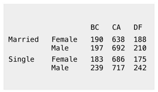
S 3568 3625We can also produce multidimensional tables based on three or more categorical variables. For this, we leverage the ftable( ) function to print the results more attractively. In this case we assess the count of customers by marital status, gender, and location:
# customer counts across location by gender and marital status

table1 <- table(supermarket$`Marital Status`, supermarket$Gender, supermarket$`State or Province`)

# Remember that the previous command is taking the table we are creating and saving it into
# a new variable called "table1". We will now take this table and evaluate it
# using the **ftable( )** command.

ftable(table1)
BC CA DF Guerrero Jalisco OR Veracruz WA Yucatan Zacatecas
M F 190 638 188 77 15 510 142 1166 200 476
M 197 692 210 94 5 514 108 1160 129 155
S F 183 686 175 107 30 607 125 1134 164 357
M 239 717 242 105 25 631 89 1107 161 309Proportions
We can also produce contingency tables that present the proportions (percentages) of each category or combination of categories. To do this we simply feed the frequency tables produced by table( ) to the prop.table( ) function. The following reproduces the previous tables but calculates the proportions rather than counts:
# Calculate the percentages of gender categories

# We will first create a new table so we don't accidentally hurt our previous work.

table2 <- table(supermarket$Gender)

# After saving the output ( new table) to the variable table2, we will now send
# this table2 to prop.table( ).

prop.table(table2)
        F         M
0.5099936 0.4900064
Based on the output, we can see that there are about 51% of respondents saying they are female (F) and about 49% of the respondents saying they are male (M).
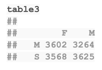
We could also create a two-way table by adding another variable. For example, let’s create a table that tallies up the variables Marital Status and Gender.
# We shall create a new table (table3) to analyze.

table3 <- table(supermarket$`Marital Status`, supermarket$Gender)

# We can now create a table of proportions for these variables.

prop.table(table3)
            F         M
  M 0.2562060 0.2321644
  S 0.2537876 0.2578420
We can interpret this tables as follows :
- 25.6% of the respondents identify as Female (F) and Married (M)
- 23.2% of the respondents identify as Male (M) and Married (M)
- 25.3% of the respondents identify as Female (F) and Single (S)
- 25.8% of the respondents identify as Male (M) and Single (S)
Note that we can tell ftable( ) how many decimal place to use when reporting the results. For example, go back to table 1. We can combine several commands together into one :
- We want to run prop.table( ) on table 1
- We want to limit to 3 decimal places
- We want to round the results
- We want to take this result and use ftable( )
ftable(round(prop.table(table1), 3)) BC CA DF Guerrero Jalisco OR Veracruz WA Yucatan Zacatecas
M F 0.014 0.045 0.013 0.005 0.001 0.036 0.010 0.083 0.014 0.034
M 0.014 0.049 0.015 0.007 0.000 0.037 0.008 0.083 0.009 0.011
S F 0.013 0.049 0.012 0.008 0.002 0.043 0.009 0.081 0.012 0.025
M 0.017 0.051 0.017 0.007 0.002 0.045 0.006 0.079 0.011 0.022Marginals
Marginals show the total counts or percentages across columns or rows in a contingency table. For instance, if we go back to table3 which is the cross classification counts for gender by marital status:
The margins are simply the sums of the rows and the columns. For example, if we look at table3, I might want to know, “How many respondents identify as Single?” This is the sum on the last row, 3568 + 3625 = 7,193. Similarly, the amount of those identifying as Married would be 3602 + 3264 = 6,866. We can calculate these values using the margin.table( ) command.
# FREQUENCY MARGINALS
# row marginals - totals for each marital status across gender

margin.table(table3, 1)
   M    S
6866 7193
# This command takes in the table for which we want to find the margins.
# The second parameter tells us if we want row (1) or column (2) margins.
We can see that this example verifes the values we calculated above.
We could also calculate the column margins by changing the second parameter to 2. It is left to you to verify that these values are correct.
# column marginals - totals for each gender across marital status

margin.table(table3, 2)
   F    M
7170 6889
If we were more interested in proportions / percentage rather than counts, we could use the prop.table( ) command to calculate these proportions. The first example will calculate the row percentages.
# PERCENTAGE MARGINALS

# row marginals - row percentages across gender

prop.table(table3, margin = 1)
            F         M
  M 0.5246140 0.4753860
  S 0.4960378 0.5039622
We could easily calcuate the column percentages using the following command.
# column marginals - column percentages across marital status

prop.table(table3, margin = 2)
            F         M
  M 0.5023710 0.4737988
  S 0.4976290 0.5262012
tabyl()
The tabyl( ) function from the janitor package is a powerful tool for creating contingency tables. It is a more modern and user-friendly version of the table( ) function. The tabyl( ) function is used to create a contingency table of counts or proportions or both!
# Make sure you install the janitor package if it is not already loaded up
# and ready to go.

# install.packages("janitor")

library(janitor)
We previously used this command to create a frequency table for the Gender variable in the supermarket data set.
table(supermarket$Gender)
We can use the tabyl() function to create the same table, along with the percentages.
t1 <- tabyl(supermarket, Gender)

t1
Gender n percent
F 7170 0.5099936
M 6889 0.4900064While we are here, let’s take a look at the structure we just created, t1.
class(t1)[1] "tabyl" "data.frame"Nice! We have created a data frame! This sets us up to more easily manipulate the data.
We can also create a two-way table by adding another variable. For example, let’s create a table that tallies up the variables Marital Status and Gender.
# Here was the code from above:

# table(supermarket$`Marital Status`, supermarket$Gender)

# Here is the code using the tabyl() function:

t2 <- tabyl(supermarket,`Marital Status`, Gender)

t2
Marital Status F M
M 3602 3264
S 3568 3625We can also add percentages to the table using the adorn_percentages( ) function. Since this is a two way table, we need to know if we want the percentages to be calculated by row or by column.
Note : We will use the pipe operator %>% to chain the functions together. We will go over this in more detail in the Beginning Data Cleaning section.
# Here is the default command. the %>% bascially means to take t2 and
# send it to the next function, adorn_percentages() :

t2 %>% adorn_percentages()
Marital Status F M
M 0.5246140 0.4753860
S 0.4960378 0.5039622This shows us that the default is to calculate the percentages by row. If we want to calculate the percentages by column, we can use the denominator parameter.
t2 %>% adorn_percentages(denominator = "col") Marital Status F M
M 0.502371 0.4737988
S 0.497629 0.5262012We can also add the counts to the table using the adorn_ns( ) function.
t2 %>% adorn_percentages(denominator = "col") %>% adorn_ns() Marital Status F M
M 0.502371 (3,602) 0.4737988 (3,264)
S 0.497629 (3,568) 0.5262012 (3,625)You can see from the output that the counts are added to the table parenthetically.
Lastly, we could add the totals (marginals) to the table using the adorn_totals( ) function.
t2 %>% adorn_percentages(denominator = "col") |> adorn_ns() Marital Status F M
M 0.502371 (3,602) 0.4737988 (3,264)
S 0.497629 (3,568) 0.5262012 (3,625)This now gives us two different methods to create contingency tables in R. tabyl() is a more modern and user-friendly version of the table() function. It can be incorporated into the dplyr workflow and is a great tool for creating contingency tables. table() is a base R function that is also useful for creating contingency tables. It is a bit more straightforward than tabyl() and is also a good tool for creating contingency tables.
Practice Problems
For this set of practice problems, you are to carry out these commands in an R script. You can use your own versino of R-Studio or you can use Post Cloud. You will be using the Arthritis data set from the vcd package.
- Install and attach the library for the package “vcd”.
Solution
# This will install the package if it is not already installed :

install.packages("vcd")

# This will attach the package to your R session.

library(vcd)- Do a Google search to describe what we are getting when we load the vcd library.
Solution
You can also use the help command to get more information about the package.
help(package = "vcd")
The vcd package is a collection of functions for visualizing categorical data.
You can also use the rdocumentation.org website to get more information about the package.
https://www.rdocumentation.org/packages/vcd/versions/1.4.8
- Describe what is in this data set (with View(Arthritis) ) and explain the variables and factors of each variable.
Solution
View(Arthritis)

# or

view(Arthritis)

# There are five variables being measured:

# ID - This is the patient's ID number
# Treatment - This tells us if the patient got the treatment or a placebo.
# Sex - This provides the gender of the patient. Limited to Female / Male.
# Age - This gives the age of the patient.
# Improved - This tells us the improvement level of the patient : None, Some
# or Marked.- Show what is in the 1st to the 17th rows of the frame “Arthritis”
Solution
# Remember in this data frame, we can call out specific rows and columns
# by limiting the rows and columns we want to see.

# This will show us the first 17 rows of the data frame.

view(Arthritis[1:17, ])

# If you notice, we get the same output using the following :

View(Arthritis[1:17, ])

# Is this always true? Check out the next rpactice problem.- Show rows 28 to 42 and only columns 2 and 5 of the frame “Arthritis”
Solution
# We could look at these one at a time :

view(Arthritis[28:42,2])

# This shows us the treatments for the fifteen patients in rows 28 to 42.

# What happens if we use `View`?

View(Arthritis[28:42,2])

# We get an output that is not very helpful! So be careful with the version
# of `view` or `View` you are using.

# We can look at the fifth column using the following :

view(Arthritis[28:42, 5])

# We could have done this with a single command by creating a vector that
# specifies which rows to use :

view(Arthritis[c(28:42), c(2,5)])

# Also note that you could print the output to the console by just typing
# the command without the `view` or `View` command.

Arthritis[c(28:42), c(2,5)]

# If needed, you could have also saved that output to another variable. Let's
# call it `results`.

results <- Arthritis[c(28:42), c(2,5)]- Show patient ID’s 1, 15, 42, and 81 and only the “Treatment” and “Improved” columns of the frame “Arthritis” using a single command.
Solution
# To specify the rows we want, we can create a vector of rows we want to use.
# In this practice problem we want to use rows 1, 15, 42 and 81.

# c(1, 15, 42, 81)

# We want to use the "Treatment" and "Improved" columns. These are columns 2 and
# 5, so we could do something similar and create a vector representing those columns.

# We could call this command :

view(Arthritis[c(1, 15, 42, 81), c(2,5)])

# Since this is a data frame, we could also used the columns names and the
# following command to get the same output :

Arthritis[c(1, 15, 42, 81), c("Treatment", "Improved")]

# While this is a little more readable and easier to understand, either method
# is acceptable.- Examine the class of each variable in Arthritis using the
str( )command and determine the summary information for Arthritis using thesummary( )command.
Tip
# Determine the class of each variable :

str(Arthritis)

# Examine the output. We see that `ID` and `Age` are numeric variables and
# the other variables are factors (categorical) variables.

# Recall that if a variable is a numeric variable, we can calculate values
# such as mean, median, sd, etc. If a variable is a factor, we can calculate
# values such as counts, proportions, etc.

# What happens when we run the summary command?

summary(Arthritis)

# We get a summary of the data frame. This is a great way to get a quick
# overview of the data frame. We can see that the categorical variables return
# the counts for each category in the data frame and the numeric variables return
# the mean, median, min, max, 1st and 3rd quartiles.

# Two things of note here :

# 1 : While we can get a summary of the numeric variable `ID`, it doesn't make
#     much sense to do so. This is a unique identifier for each patient and
#     is not particulary useful in any analysis.

# 2 : We will go over in much greater detail the meanings of the quartiles and
#     the other summary statistics in Part 4 of this text. For now, just know that
# these are useful values to know about the data frame.- Show the values of the “Treatment” column for “Arthritis”. Try using the
str( )command and thesummary( )command.
Solution
# We could use `str( )` or `summary( )` to do this for us.

str(Arthritis$Treatment)

# If you examine the output :

# Factor w/ 2 levels "Placebo","Treated": 2 2 2 2 2 2 2 2 2 2 ...

# We see that the variable `Treatment` is a factor with 2 levels. The levels
# are "Placebo" and "Treated".

# We can also use the `summary( )` command to get the counts for each level.

summary(Arthritis$Treatment)

# This gives us a little more helpful information.

# Placebo Treated
#      43      41

# We can see the treatments and also the count for each treatment.- Show the levels of the “Treatment” column for “Arthritis”. (Hint : levels command…..)
Solution
# We can also use the `levels( )` command to get the levels of the factor.

levels(Arthritis$Treatment)

# This output is useful if we only care about the names of the treatments.

# [1] "Placebo" "Treated"- Use the length( ) function to find the number of patients in “Arthritis”
Solution
# We can use the `length( )` function to find the number of patients in the data frame.
# But be careful with how you call the command.

# What happens if we call `length(Arthritis)`?

length(Arthritis)

# [1] 5

# This will give us the number of variables (columns) in the data frame, which
# from the output is 5. This is not what we want.

# What we should do is see the length of the number of IDs in the data frame.

length(Arthritis$ID)

# [1] 84

# This gives us the number of patients (rows) in the data frame, which is 84.
- Use the table( ) function to display the tabulated results for the “Improved” column of “Arthritis” (Note the summary( ) function does the same thing). Put the result in the variable “ImprovedTable”.
Solution
# We can use the `table( )` function to get the counts for each level of the factor.

# We will save the output to a new variable called `ImprovedTable`.

ImprovedTable <- table(Arthritis$Improved)

# This will give us the counts for each level of the factor.

view(ImprovedTable)

#   None   Some Marked
#     42     14     28

# We can also use the `summary( )` function to get the counts for each level of the factor.

summary(Arthritis$Improved)

#   None   Some Marked
#     42     14     28
- Use the prop.table( ) function on ImprovedTable to get a table of proportions
Solution
# We can use the `prop.table( )` function to get the proportions for each level of the factor.

# We will save the output to a new variable called `ImprovedTableProp`.

ImprovedTableProp <- prop.table(ImprovedTable)

# This will give us the proportions for each level of the factor.

view(ImprovedTableProp)

#      None      Some    Marked
# 0.5000000 0.1666667 0.3333333

# We can verify these values by dividing the counts by the total number of patients.
# We found that a few steps ago and saw we had 84 patients.

# Here were those results :

#   None   Some Marked
#     42     14     28

# This leads to the proportions :

# 42 / 84 = 0.5000000
# 14 / 84 = 0.1666667
# 28 / 84 = 0.3333333

# Being able to verify small examples is a good habit to get into. It helps you
# understand the data and also helps you understand the code you are writing and
# that it is correct.
- Use the xtabs( ) function to cross-tabulate “Treatment” versus “Improved” in the “Arthritis” data frame. Call the result “Treat.Improv”.
Solution
# We can use the `xtabs( )` function to cross-tabulate the two variables.

xtabs(~ Treatment + Improved, data = Arthritis)

# This leads to a nice output in the console :

#          Improved
# Treatment None Some Marked
#   Placebo   29    7      7
#   Treated   13    7     21

# Here we have a nice two-way table that shows the counts for each combination of
# Treatment and Improved. For example, the 21 represents the number of patients
# that were treated and had a marked improvement. The 29 represents the number of
# patients that were given a placebo and had no improvement.

# We will save the output to a new variable called `Treat.Improv`.

Treat.Improv <- xtabs(~ Treatment + Improved, data = Arthritis)

# We have several different ways to view this data, so experiment and
# find the one that works best for you.

# We can also use the `ftable( )` function to get a more readable output.

ftable(Treat.Improv)

#           Improved None Some Marked
# Treatment
# Placebo              29    7      7
# Treated              13    7     21


# We can also use the `table( )` function :

table(Treat.Improv)

# Treat.Improv
#  7 13 21 29
#  3  1  1  1

# Unfortunately, this is not very helpful unless we already know the variables
# and the order of the levels.

# Lastly, we could use view and View. They return the same output which is not
# presented as a two-way table, but in tidy data format!

view(Treat.Improv)
- Add marginal sums to the table
Treat.Improvusing the addmargins( ) function.
Solution
# We can use the `addmargins( )` function to add the marginal sums to the table.

addmargins(Treat.Improv)

# This will give us the following output :
#          Improved
# Treatment None Some Marked Sum
#   Placebo   29    7      7  43
#   Treated   13    7     21  41
#   Sum       42   14     28  84

# We can also use the `ftable( )` function to get a slightly more readable output.

ftable(addmargins(Treat.Improv))

#           Improved None Some Marked Sum
# Treatment
# Placebo              29    7      7  43
# Treated              13    7     21  41
# Sum                  42   14     28  84

# We can also use the `table( )` function, but again the output is not as nice:

table(addmargins(Treat.Improv))

#  7 13 14 21 28 29 41 42 43 84
# 3 1 1 1 1 1 1 1 1 1 - Create 3 tables of proportions using
Treat.Improv: proportion of total, proportion of row sum, and proportion of column sum. Call the 3 tables: P.Table1, P.Table2, and P.Table3 and use three decimal places of accuracy.
Solution
# We can use the `prop.table( )` function to get the proportions for each level of the factor. We will deal with accuracy in a bit.

# We will save the output to a new variable called `P.Table1`.

P.Table1 <- prop.table(Treat.Improv)             # proportion to total

# This will give us the proportions for each level of the factor.

#          Improved
# Treatment       None       Some     Marked
#   Placebo 0.34523810 0.08333333 0.08333333
#   Treated 0.15476190 0.08333333 0.25000000

P.Table2 <- prop.table(Treat.Improv, margin = 1).  # proportion to row sum

#          Improved
# Treatment      None      Some    Marked
#   Placebo 0.6744186 0.1627907 0.1627907
#   Treated 0.3170732 0.1707317 0.5121951


P.Table3 <- prop.table(Treat.Improv, margin = 2)   # proportion to column sum

#          Improved
# Treatment      None      Some    Marked
#   Placebo 0.6904762 0.5000000 0.2500000
#   Treated 0.3095238 0.5000000 0.7500000


# We can also use the `ftable( )` function to get a more readable output.

ftable(P.Table1)

#           Improved None      Some     Marked
# Treatment
# Placebo              0.3452381 0.08333333 0.08333333
# Treated              0.1547619 0.08333333 0.25
# Sum                  0.5       0.16666667 0.33333333

# We can also use the `table( )` function, but again the output is not as nice:
table(P.Table1)

# We can now use a combination of `round` and `ftable` to get the output we want.
# Recall we want 3 decimal places of accuracy, and that is the parameter at the
# end of the command.

ftable(round(P.Table1, 3))

#           Improved  None  Some Marked
# Treatment
# Placebo            0.345 0.083  0.083
# Treated            0.155 0.083  0.250

ftable(round(P.Table2, 3))

#           Improved  None  Some Marked
# Treatment
# Placebo            0.674 0.163  0.163
# Treated            0.317 0.171  0.512

ftable(round(P.Table3, 3))

#           Improved  None  Some Marked
# Treatment
# Placebo            0.690 0.500  0.250
# Treated            0.310 0.500  0.750

# Note that we could have done this in one command :

ftable(round(P.Table3, 3))
ftable(round(prop.table(Treat.Improv, margin=1), 3))
ftable(round(prop.table(Treat.Improv, margin=2), 3))