library(tidyverse)
x <- 1:10
y <- x^2
df = data.frame(x, y)
ggplot(df,
aes(x = x, y = y)) +
geom_point()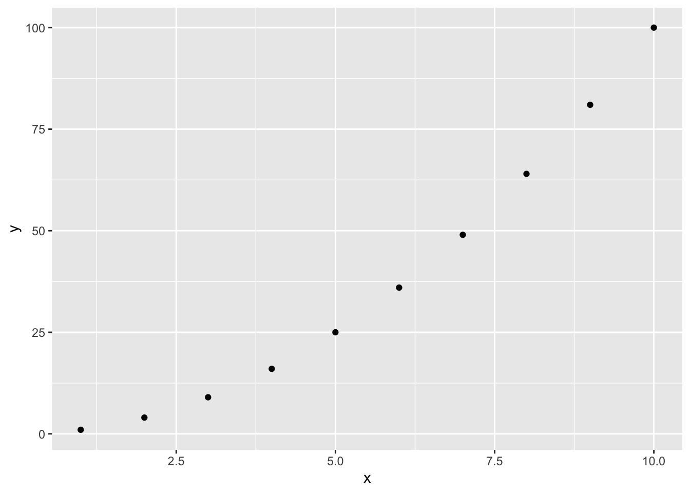
Now that we have seen many different tools we can use to analyze our data, we can start to think about how we can present our findings. In this section, we will look at how we can create documents and reports using Quarto documents.
A Quarto document is a file that contains both text and code. The text is written in Markdown, which is a lightweight markup language that is easy to read and write. The code is written in R, and it can be used to generate plots, tables, and other outputs.
Let’s first talk about what makes up a Quarto document. For our purposes, there are three parts to know.
YAML Header - This is the first part of the document. It contains metadata about the document, such as the title, author, and date.
Text - This is the main part of the document. It contains the content of the document, such as text, code, and outputs.
Code Chunks - These are sections of code that can be executed. They are enclosed in three backticks (```) and can contain R code.
We will walk through each of these three parts in more detail, but first let’s see how we can use R Studio to create a Quarto document.
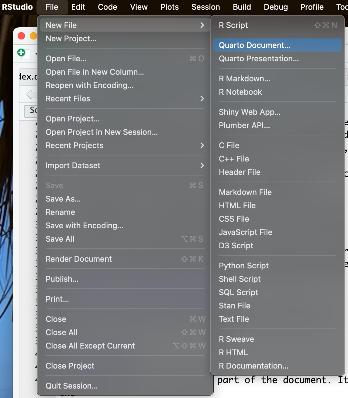
To create a Quarto document, we can use R Studio. In R Studio, we can go to File > New File > Quarto Document.
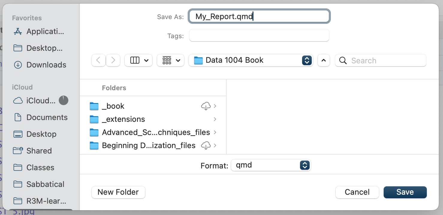
You will be then prompted to enter a title and author of your document. As you can see below,
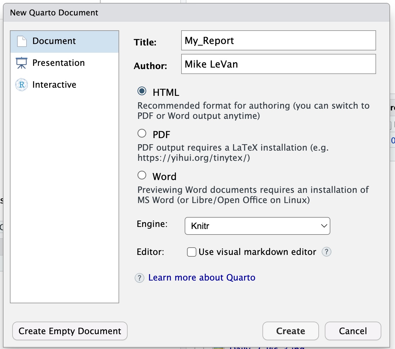
(Note that this is not the same as saving your file to your working directory. We will do that in a few steps.)
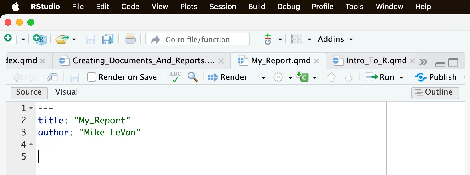
This will create a new Quarto document with a default YAML header.
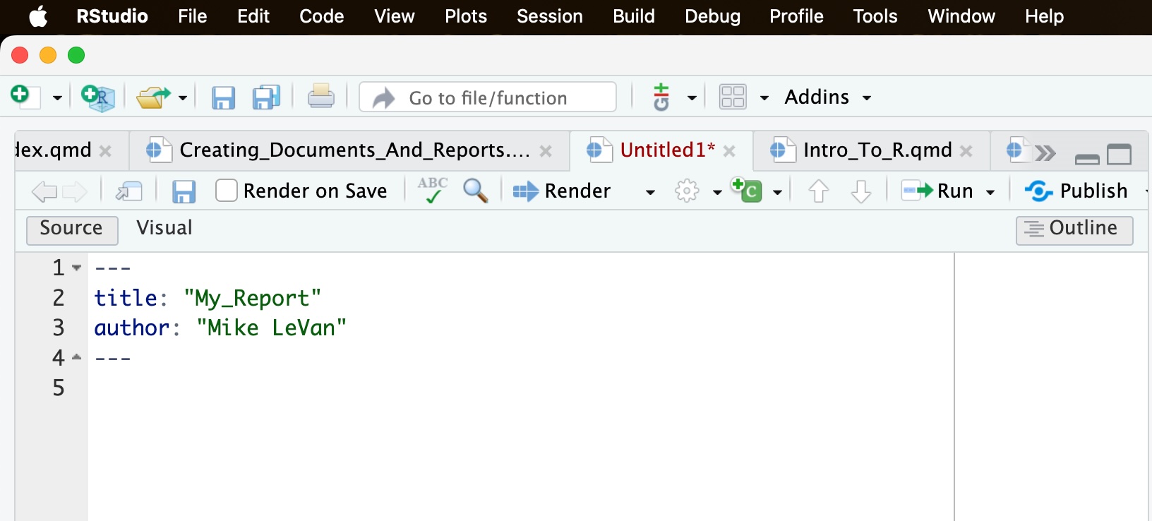
There are a few things to note about the Quarto document.
You have a choice in how you edit the document. You cab click on the Source or Visual button to choose your editor. markdown editor. I prefer the source editor, but you can use either one. The examples are assuming you are using the source editor.
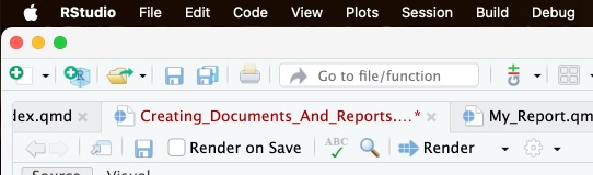
Notice the tab we are working in. It is called Untitled1*. This is the name of the file we are working in. You can change the name of the file by going to File > Save As and entering a new name. I will name my file “My_Report.qmd”. You can name your file whatever you like, but make sure to use the “.qmd” extension and are saving to the appropriate directory.
We are now ready to start editing our document! Let’s walk through the three parts of the document.
While there are many different customizations one can use in this header, we are just oging to highlight some basic properties. For more information on the YAML header, see the Quarto documentation.
The YAML header is the first part of the document. It contains metadata about the document, such as the title, author, and date. It also contains information about the output format, such as HTML, PDF or Word. The YAML header is enclosed in three dashes (—) at the beginning and end.
Here is an example of a YAML header:
---

title: "Creating Documents and Reports"
author: "Mike LeVan"
date: "2025-12-19"
output: html_document
---
Let’s go through each part of the given YAML header.
title: This is the title of the document. You can enter any title you like.author: This is the author of the document. You can enter your name or any name you like.date: This is the date of the document. You can enter any date you like. The 2025-12-19 command will automatically enter the current date.output: This is the output format of the document. You can choose from HTML, PDF, Word, and many other formats. For this document, we will use HTML.The text is the main part of the document. It contains the content of the document, such as text, code, and outputs. The text is written in mostly plain text, but there are some Markdown syntax that you can use to format the text.
Here are some examples of Markdown syntax:
# for headings## for subheadings* for bullet points1. for numbered lists** for bold text* for italic textYou can create headings by using the # symbol. The number of # symbols indicates the level of the heading. For example, # is a level 1 heading, ## is a level 2 heading, and so on. This can go down to 6 levels.
# This is a level 1 heading

## This is a level 2 heading

### This is a level 3 headingYou can create bullet points by using the * symbol. For example if we write the following in a Quarto document:
* This is a bullet point

* This is another bullet point

* This is a third bullet point
We will get the following output:
You can create numbered lists by using the 1. symbol. For example if we write the following in a Quarto document:
1. This is a numbered list

2. This is another numbered list

3. This is a third numbered list
We will get the following output:
You can start the list with any number you like. The numbers will be automatically updated when you render the document. Consider this code:
7. This is a numbered list

8. This is another numbered list

9. This is a third numbered list
This will lead to the following output:
The only important value is the first one. The rest will be updated when you render the document. Look at this example:
19. This is a numbered list

8. This is another numbered list

13. This is a third numbered list
This command will generate the following list :
You can create bold text by using the ** symbol around the text you want to put in bold. For example if we write the following in a Quarto document:
**This is bold text**We will get the following output:
This is bold text
You can create italic text by using the * symbol around the text you want to italicize. For example if we write the following in a Quarto document:
*This is italic text*We will get the following output:
This is italic text
Quarto will try to format the spacing for you. Consider this code:
This is a line
of text.
This will lead to the following output:
This is a line of text.
Notice that it ignored the new line and tried to put the text on one line. If you want to force a new line, you can use the <br> tag. For example if we write the following in a Quarto document:
This is a line <br>
of text.
We will get the following output:
This is a line
of text.
You can leave blank lines between paragraphs to create space. For example if we write the following in a Quarto document:
This is a line of text.

This is another line of text.
We will get the following output:
This is a line of text.
This is another line of text.
You can add images to your document by using the following syntax :

The ! is for the image, the [] is for the alt text and the () is for the image path. For example if we write the following in a Quarto document:
The above code is assuming I have a directory called “images” in the same directory as my Quarto document and that I have an image called “Pic_1.jpg” in that directory. The image will be displayed in the document. If there is no image, the Alternate Text will be displayed.
There are going to be times when you have completed your data anlysis and you want to display the results in a table. You can do this firly easily using Quarto.
Let’s say you have done some research and have data that contains the top 5 home run hitters of all time from the Cincinnati Reds. Here is how we would like to display the data:
| Player Name | Home Runs |
|---|---|
| Johnny Bench | 389 |
| Joey Votto | 356 |
| Frank Robinson | 324 |
| Tony Perez | 287 |
| Adam Dunn | 270 |
This is done without using any R code. This table was created in the Quarto document using the following syntax as just plain text:
| Player Name     | Home Runs|
|:----------------|:--------:|
| Johnny Bench    |    389   |
| Joey Votto      |    356   |
| Frank Robinson  |    324   |
| Tony Perez      |    287   |
| Adam Dunn       |    270   |
There are some other options you can use to format the table. For example, you can justify the text in the columns. Look at the second column of the table above. The combination of the colon (:) and the dashes (-) give the justification.
|:---------| means left justify the text in that column.|---------:| means right justify the text in that column.|:---------:| means center justify the text in that column.If we look at the previous example, the first column is left justified, the second column is center justified.
The widths of the columns is proportional to the number of dashes (-) in the header. In our example we have 16 dashses in the first column and 8 dashes in the second column. This means the first column will be twice as wide as the second column. If we change the number of dashes in the header, we can change the width of the columns. For example if we write the following in a Quarto document:
| Player Name   | Home Runs |
|:------------  |:------------:|
| Johnny Bench  |    389    |
| Joey Votto    |    356    |
We will get a table that has 50% of the table width for the first column and 50% of the table width for the second column. This is because we have the same number of dashes in both columns (12 dashes).
| Player Name | Home Runs |
|---|---|
| Johnny Bench | 389 |
| Joey Votto | 356 |
We can add captions to the table by using the following syntax:
| Player Name   | Home Runs |
|:------------  |:------------:|
| Johnny Bench  |    389    |
| Joey Votto    |    356    |

: HR Hitters
This will add a caption to the table that says “HR Hitters”. The caption is added after the table and is preceded by a colon (:).
| Player Name | Home Runs |
|---|---|
| Johnny Bench | 389 |
| Joey Votto | 356 |
We can also use bold and italic text in the table using the methods we saw above.
| Player Name   | Home Runs |
|:------------  |:------------:|
| Johnny Bench  |    389    |
| Joey Votto    |    356    |

: **HR Hitters**| Player Name | Home Runs |
|---|---|
| Johnny Bench | 389 |
| Joey Votto | 356 |
For a more complete overview of how to create tables in Quarto, see the Quarto documentation.
What is really nice about Quarto documents is that you can include code chunks in the document. This allows you to run R code and include the output in the document. This is really useful for creating reports and documents that include data analysis and visualizations.
A code chunk is enclosed in three backticks (```) and can contain R code. For example if we write the following in a Quarto document:
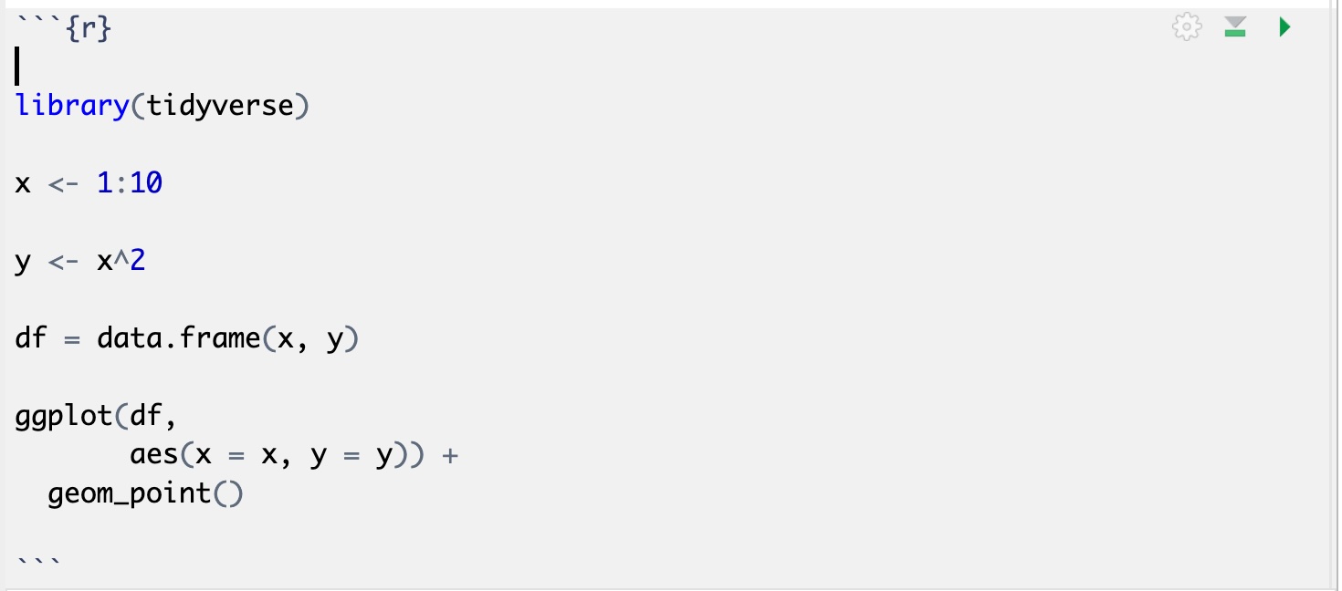
We will get the following output:
library(tidyverse)

x <- 1:10

y <- x^2

df = data.frame(x, y)

ggplot(df,
       aes(x = x, y = y)) +
  geom_point()
Which is GREAT because now we can work out all the details and visualizations needed in an R script, and then just copy and paste the code into the Quarto document.
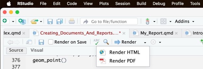
Once you have finished writing your document, you can render it to the output format you chose in the YAML header. To render the document, you can click on the Render button in the toolbar or go to the menu and select Render.
There are some options you can take advantage of when rendering your document. For example, if you click on the little arrow next to the Render button, you can choose to render the document to a different format, such as PDF.
You can also choose where you want to view the output. You can click on the arrow next to the gear icon to choose to view the output in the Viewer pane or in the web browser.
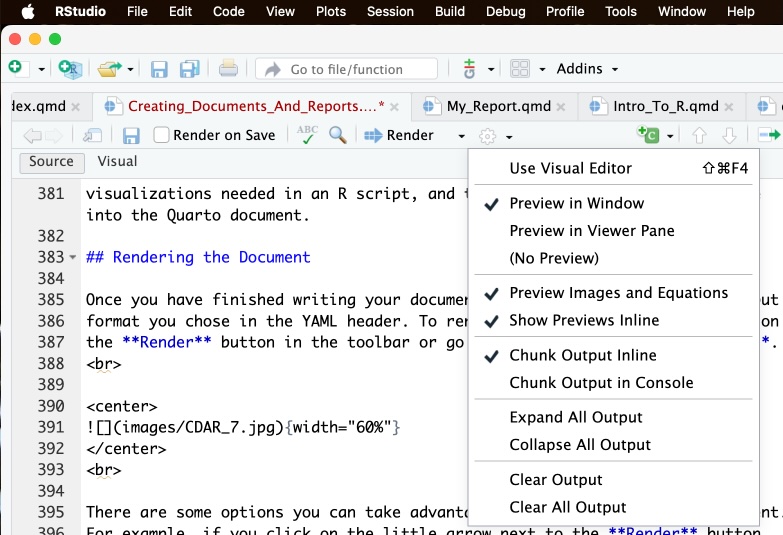
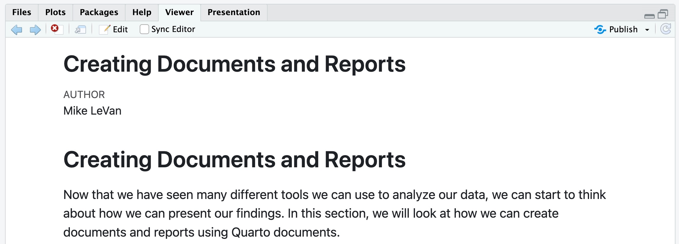
If you choose “Preview in Window”, then the output will show up in a web broswer.
If you choose “Preview in Viewer Pane, then the output will show up in the Viewer pane in R Studio.
This is just the beginning of what you can do with Quarto documents. There are many other features and options that you can use to customize your documents.