# Read in the data

Reds2024_Another_Version <- read.csv("./Reds-2024.csv")

# CAUTION : When creating variable names to use in your R script,
# make sure you use an underscore and not a dash. When R sees a dash,
# it can sometimes be interpreted as a minus sign and not a dash.
# This can cause errors in your code.

# You can try this by removing the comment tag below :

# Reds-2024 <- read.csv("Reds-2024.csv")Reading In Data
We have seen a few different ways for us to store data. We discussed Vectors, Data Frames and Tibbles. We now move on to the question of how we can get data from a file into R so we can start some Elementary Data Analysis, Visualization, and other fun stuff!
CSV Files
Let’s consider the case to where we have data in a CSV file. If you are unaware, CSV stands for “comma separated values.” These are simple text files where the data is separated by commas. We can use the read.csv() or read_csv()function to read the data into a variable in R.
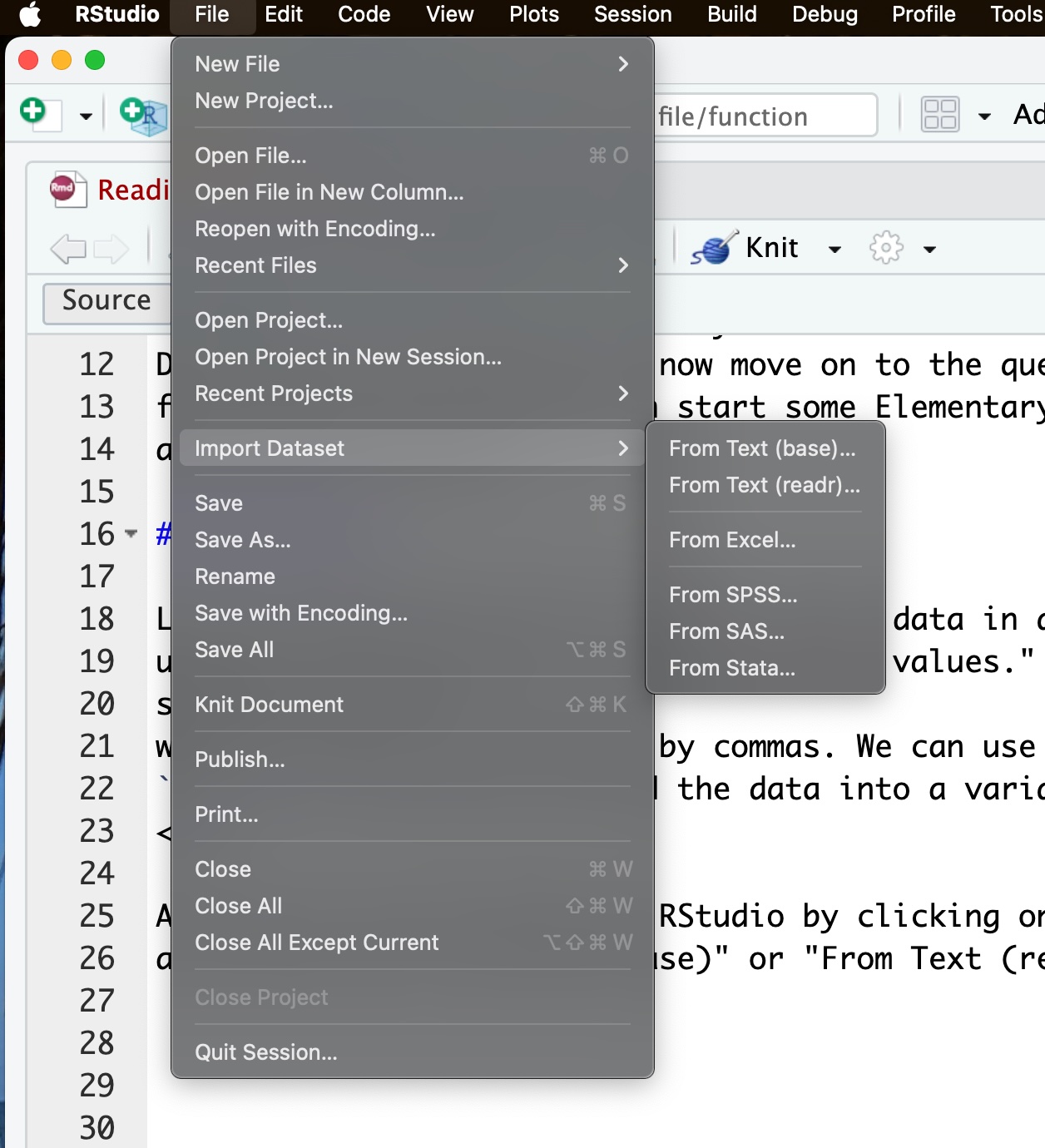
A CSV file can be upload to RStudio by clicking on “File” and then “Import Dataset” button and selecting “From Text (base)” or “From Text (readr).”
For this particular example, I asked ChatGPT to create a CSV file for me using the following query :
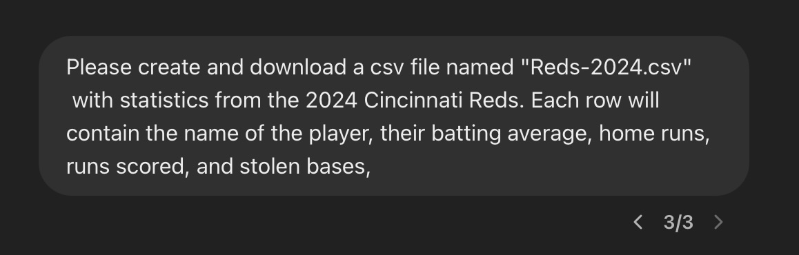
You can download the file here :
Once I had the file downloaded, I then proceeded to upload it using the steps above. (Make sure you know which directory the file was sent to when it was downloaded!) First, I went to :
Files ->
Import Dataset ->
From Text (readr)
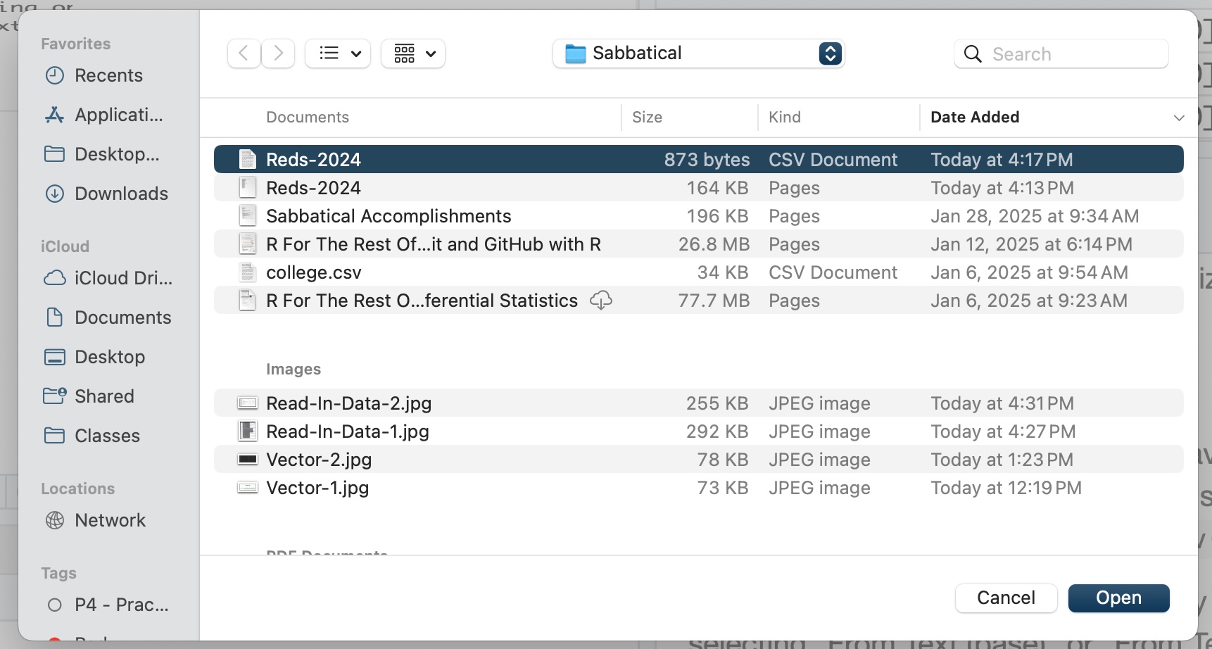
This gave me a new dialog and I clicked on the file Reds-2024. Notice that I picked the CSV version and not the Pages version!
I then clicked on the “Import” button and a new dialog was presented to me :
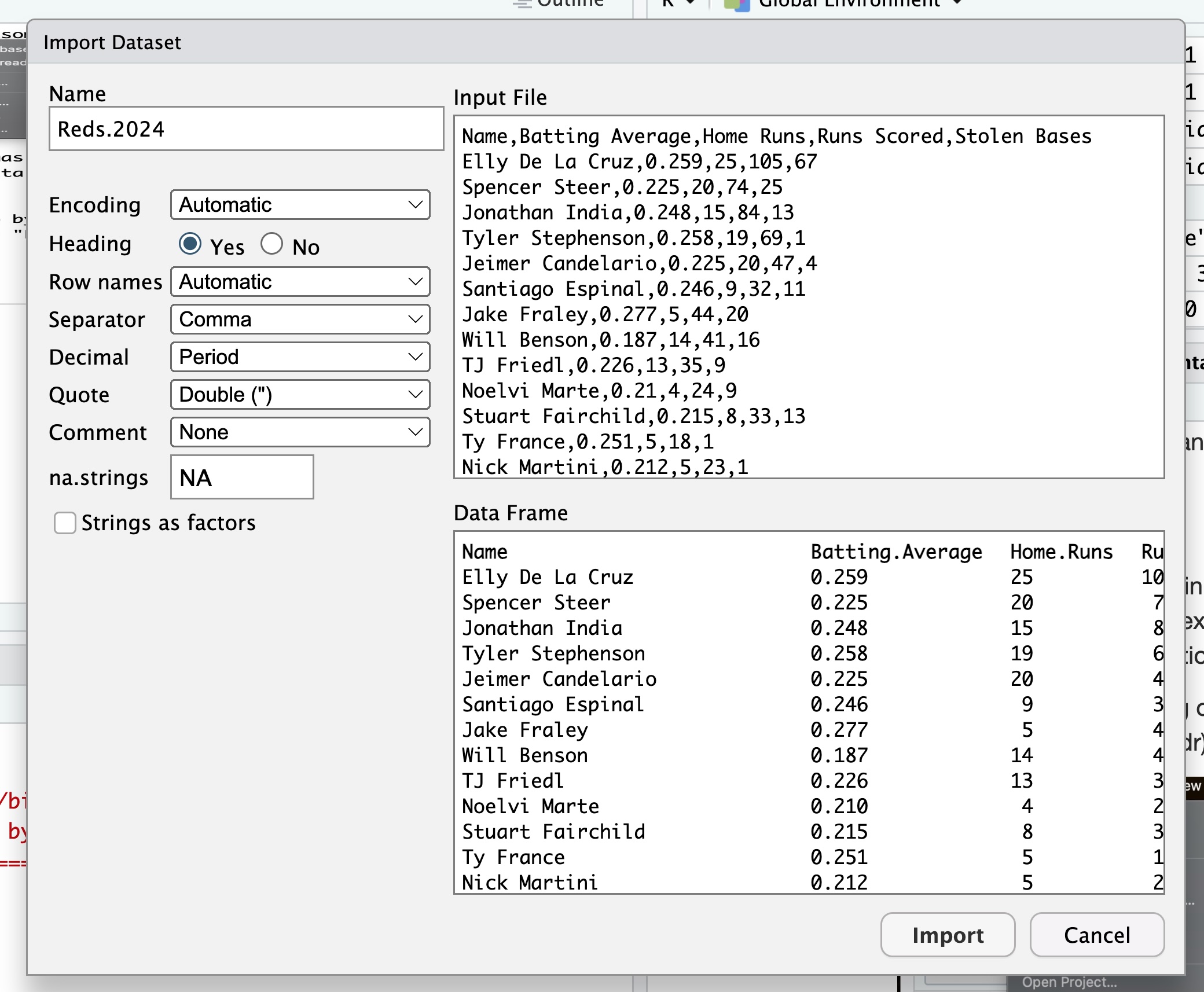
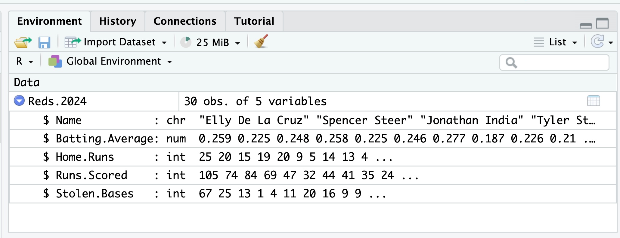
If you look in the upper left hand corner, you will see that you are given a choice for the name of your file. The default one given is Reds.2024, but you can change that to anything you wish. I went ahead and just kept this default name. I clicked on the “Import” button and the data was loaded into RStudio into the variable Reds.2024. You can look at the variable in the Environment tab :
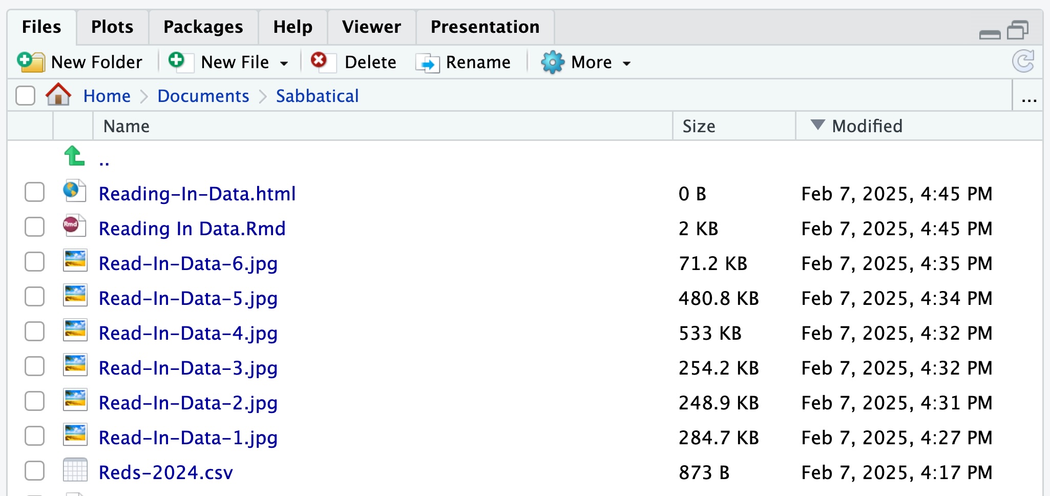
You can also see the CSV file in the Files tab :
Data Organization
As you progress in your skills, you will find that organizing your data is very important. A good practice is to keep your data files in a separate folder from your R scripts. This way, you can easily find your data files and your R scripts. You can also create subfolders for different projects or datasets.
read.csv( )
We can write part of our code to read in a CSV file using the read.csv() function. The read.csv() function takes in a file path as an argument. If you have a CSV file uploaded into the files section of RStudio, you can use the read.csv() function :
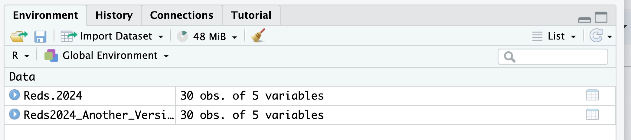
We can now see the new version of the data in the Environment tab :
read.csv() is a base R function. That means it is already loaded up when you start RStudio. You do not need to load any packages to use it.
However, there is a more powerful function called read_csv() that is part of the readr package. It can read in data faster and it can also read in data that is not in a CSV format, but we will stick with the CSV format for now.
read_csv( )
One of the differences between read.csv( ) and read_csv( ) is that read_csv( ) is part of the readr package. This means you will need to load the readr package to use it. This is part of the tidyverse package. If you do not have tidyverse installed, make sure you go ahead and install it. Once tidyverse is install, you can load up the readr package.
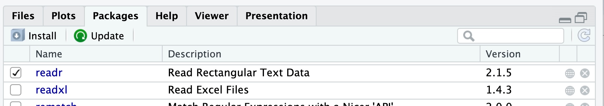
If you are unsure if the readr package is loaded, you can look at the Packages tab in RStudio to see if the readr package is loaded. If it is not, you can load it by clicking on the checkbox next to the package name.
If needed, you can also put this into your script so the user will have it loaded up for them. You can load the readr package by using the library() function :
# Load the readr package

library(readr)
You can now use the read_csv() function to read in the data :
# Read in the data. We will read in the csv file "Reds-2024.csv" and
# store it in the variable Reds2024_Version_3.

Reds2024_Version_3 <- read_csv("Reds-2024.csv")
Rows: 30 Columns: 5
── Column specification ────────────────────────────────────────────────────────
Delimiter: ","
chr (1): Name
dbl (4): Batting Average, Home Runs, Runs Scored, Stolen Bases
ℹ Use `spec()` to retrieve the full column specification for this data.
ℹ Specify the column types or set `show_col_types = FALSE` to quiet this message.Why is read_csv better than read.csv? It is faster and it can read in data that is not in a CSV format. It can read in data that is in a TSV (Tab Separated Value) format, a DSV (Delimiter Separated Value) format, and a few others. It can also read in data that is in a fixed width format.
Basically, when in doubt, use read_csv( ) instead of read.csv( ).
Now that we have the data loaded into R, we can start to do some Elementary Data Analysis. We can use all the commands we discussed when going over Vectors, Data Frames, and Tibbles.
# Look at the data. The "head" command looks at the information in the
# front of the data frame. By default, it will show the first 6 rows of
# the data.

head(Reds2024_Version_3)
# A tibble: 6 × 5
Name `Batting Average` `Home Runs` `Runs Scored` `Stolen Bases`
<chr> <dbl> <dbl> <dbl> <dbl>
1 Elly De La Cruz 0.259 25 105 67
2 Spencer Steer 0.225 20 74 25
3 Jonathan India 0.248 15 84 13
4 Tyler Stephenson 0.258 19 69 1
5 Jeimer Candelario 0.225 20 47 4
6 Santiago Espinal 0.246 9 32 11# Look at the structure of the data. We can do this with the "class"
# command.
class(Reds2024_Version_3)[1] "spec_tbl_df" "tbl_df" "tbl" "data.frame" # Look at the Stolen Bases category. This command will print out all the
# values in the "Stolen Bases" column of the data frame.
Reds2024_Version_3$`Stolen Bases` [1] 67 25 13 1 4 11 20 16 9 9 13 1 1 2 0 0 3 2 2 2 0 0 0 5 0
[26] 0 1 0 0 0Using URL’s
You can also read in data from a URL. This is useful if you have a CSV file hosted on a website. You can use the read.csv() os read_csv() functions to read in the data from the URL.
If there is a direct URL to a CSV sheet, then you can use one of these commands to read in the data. The first is read.csv(). The syntax is basically dataframe_name <- read.csv('URL')
# Here we will read in a CSV file and save it to the variable "data1"

data1 <- read.csv('https://www.stats.govt.nz/assets/Uploads/Annual-enterprise-survey/Annual-enterprise-survey-2020-financial-year-provisional/Download-data/annual-enterprise-survey-2020-financial-year-provisional-csv.csv')

# We can now check out the first couple of rows to make sure it looks OK.

head(data1,2)
Year Industry_aggregation_NZSIOC Industry_code_NZSIOC Industry_name_NZSIOC
1 2020 Level 1 99999 All industries
2 2020 Level 1 99999 All industries
Units Variable_code
1 Dollars (millions) H01
2 Dollars (millions) H04
Variable_name Variable_category Value
1 Total income Financial performance 733,258
2 Sales, government funding, grants and subsidies Financial performance 660,630
Industry_code_ANZSIC06
1 ANZSIC06 divisions A-S (excluding classes K6330, L6711, O7552, O760, O771, O772, S9540, S9601, S9602, and S9603)
2 ANZSIC06 divisions A-S (excluding classes K6330, L6711, O7552, O760, O771, O772, S9540, S9601, S9602, and S9603)The second is read_csv(). The syntax is the same as above : dataframe_name <- read_csv('URL')
# Here we will read in a CSV file and save it to the variable "data2"

data2 <- read_csv('https://www.stats.govt.nz/assets/Uploads/Annual-enterprise-survey/Annual-enterprise-survey-2020-financial-year-provisional/Download-data/annual-enterprise-survey-2020-financial-year-provisional-csv.csv')
Rows: 37080 Columns: 10
── Column specification ────────────────────────────────────────────────────────
Delimiter: ","
chr (9): Industry_aggregation_NZSIOC, Industry_code_NZSIOC, Industry_name_NZ...
dbl (1): Year
ℹ Use `spec()` to retrieve the full column specification for this data.
ℹ Specify the column types or set `show_col_types = FALSE` to quiet this message.# Again, look at the data to make sure it looks OK.
head(data2,2)# A tibble: 2 × 10
Year Industry_aggregation_N…¹ Industry_code_NZSIOC Industry_name_NZSIOC Units
<dbl> <chr> <chr> <chr> <chr>
1 2020 Level 1 99999 All industries Doll…
2 2020 Level 1 99999 All industries Doll…
# ℹ abbreviated name: ¹Industry_aggregation_NZSIOC
# ℹ 5 more variables: Variable_code <chr>, Variable_name <chr>,
# Variable_category <chr>, Value <chr>, Industry_code_ANZSIC06 <chr>Note : As of now, there is not an easy way to read in data from a Google Drive. You can try to use the googledrive package, but for our purposes, if we have a csv file on Google Drive, we will download the file and upload it as we did earlier.
Excel Files
We can also read in data from an Excel file. We can use the readxl package to read in the data. If you do not have the readxl package installed, you can install it by using the install.packages() function :
# Install the readxl package

# install.packages("readxl")
You can then load the readxl package by using the library() function :
# Load the readxl package

library(readxl)
You can then use the read_excel() function to read in data. Here is an excel sheet you can download and use for this example :
You can download the file and then upload it to your RStudio project. Once you have the file uploaded, you can read in the data using the read_excel() function. The syntax is similar to the read.csv() and read_csv() functions :
# Read in the data

data3 <- read_excel("Reds_1_Excel.xlsx")

head(data3,2)
# A tibble: 2 × 5
Name `Batting Average` `Home Runs` `Runs Scored` `Stolen Bases`
<chr> <dbl> <dbl> <dbl> <dbl>
1 Elly De La Cruz 0.259 25 105 67
2 Spencer Steer 0.225 20 74 25This allows to now carry out some EDA on the variable data3. For example, if we wanted to sum up the number of home runs hit by the Reds in 2024, we could use the following code :
# Sum up the number of home runs hit by the Reds in 2024

sum(data3$`Home Runs`)
[1] 174Excel Files with Multiple Tabs
We can also read in data from an Excel file that has multiple tabs. We can use the read_excel() function to read in the data from a specific tab. The syntax is similar to the read.csv() and read_csv() functions, but we need to specify the sheet name or index.
For example, if we have an Excel file with two tabs, “Sheet1” and “Sheet2”, we can read in the data from “Sheet1” using the following code :
# Read in the data from Sheet1

data4 <- read_excel("Reds_1_Excel.xlsx", sheet = "Sheet1")

# Read in the data from Sheet2

data5 <- read_excel("Reds_1_Excel.xlsx", sheet = "Sheet2")
Here is an example of an Excel file with multiple tabs that you can download and use for this example :
This spreadsheet has 4 tabs, one for each year from 2021 to 2024. You can download the file and then upload it to your RStudio project. Once you have the file uploaded, you can read in the data from a specific tab using the read_excel() function. For example, if you want to read in the data from the 2024 tab and the 2011 tab, you can use the following code :
# Read in the data from the 2024 tab

data_2024 <- read_excel("MLBTeam_Batting_Stats_2021_2024.xlsx", sheet = "2024")

# Read in the data from the 2021 tab

data_2021 <- read_excel("MLBTeam_Batting_Stats_2021_2024.xlsx", sheet = "2021")
You now have two new data frames that you can analyse!
Installing Databases
We will be working with a database from the Star Wars universe. We need to first install the package. We can do that in a script using the install.packages command :
# Type the command below to install the "starwarsdb" package. Ignore the hashtag
# in front of the command. This is just to prevent it from running automatically.

# install.packages("starwarsdb")
This will load up a database of information about the Star Wars universe. It can be accessed by using the starwars variable. You can check this by typing in the command below :
# Type the command below to see the starwars variable.

# starwars
Please make note that this is a different kind of way we can enter data into R. We have loaded up what is called a “database” which is different from a text file, a dataframe, a tibble, etc.
There are several ways to access this data. We use the “dplyr” library to access this data, so install it if it is not already installed.
# Type the command below to install the "dplyr" package.

# install.packages("dplyr")
dplyr should now be installed, but may not be loaded. You can load the library by checking it off in the packages tab, or you can enter the following :
# Type the command below to load the "dplyr" package.

# library(dplyr)

# Notice there are not quotes around the name of the package
# for this command.
We are now ready to create a dataframe using a combination of “dplyr” and the “as.data.frame” command. This is similar to the “as.tibble” command used above. Let’s store the information in the variable starwars_DF :
# starwars_DF <- as.data.frame(starwars)


# head(starwars_DF)
Check the variable to make sure it is a dataframe.
# class(starwars_DF)
Since this is a data frame, we can now use all the commands we have learned so far to access the data.
Practice Problems
- Turn
starwars_DFinto a tibble named SW_tibble.
# Load the dplyr package

library(_______)

# Convert starwars_DF into a tibble and save it to SW_tibble

SW_tibble <- as_tibble(__________)

# Check to make sure this is now a tibble

class(_________)
Solution
# Load the dplyr package

library(dplyr)

# Convert starwars_DF into a tibble and save it to SW_tibble

SW_tibble <- as_tibble(starwars_DF)

# Check to make sure this is now a tibble

class(SW_tibble)
2. Download the file Reds_1_Excel.xlsx from the download button above. Then place it in your working directory and load it into an R script under the variable name Reds_1_Excel. From there, sum up the total number of stolen bases for the Reds in 2024.
# Load the readxl package

library(_______)

# Read in the data from the Excel file

Reds_1_Excel <- read_excel("Reds_1_Excel.xlsx")

# Sum up the total number of stolen bases for the Reds in 2024

total_stolen_bases <- sum(________$`Stolen Bases`)
Solution
# Load the readxl package

library(readxl)

# Read in the data from the Excel file

Reds_1_Excel <- read_excel("Reds_1_Excel.xlsx")

# Sum up the total number of stolen bases for the Reds in 2024

total_stolen_bases <- sum(Reds_1_Excel$`Stolen Bases`)- Download the file
student_test_scores.csvfrom the download button below. The file contains the test scores of students in a class. Upload the file to your RStudio project. Save the file to the variable calledStudent_Test_Scoresand read it in using theread_csv()function. The file contains names and test scores for 20 students. Check to make sure the data was entered propoerly.
# Load the readr package

library(_______)

# Read in the data from the CSV file

Student_Test_Scores <- read_csv("student_test_scores.csv")

# Check the data to make sure it was entered properly

head(__________)
Solution
# Load the readr package

library(readr)

# Read in the data from the CSV file

Student_Test_Scores <- read_csv("student_test_scores.csv")

# Check the data to make sure it was entered properly

head(Student_Test_Scores)- Download the file
kentucky_county_median_home_prices_2024.csvfrom the download button below. Upload the file to your RStudio project. Save the file to the variable calledKentucky_Home_Pricesand read it in using theread_csv()function. The file contains the median home prices for each county in Kentucky for 2024. Check to make sure the data was entered properly.
# Load the readr package

library(_______)

# Read in the data from the CSV file

Kentucky_Home_Prices <- ________("kentucky_county_median_home_prices_2024.csv")

# Check the data to make sure it was entered properly

head(__________)
Solution
# Load the readr package

library(readr)

# Read in the data from the CSV file

Kentucky_Home_Prices <- read_csv("kentucky_county_median_home_prices_2024.csv")

# Check the data to make sure it was entered properly

head(Kentucky_Home_Prices)- Downlad the file
hate_crimes_by_state_2024.xlsxfrom the download button below. Upload the file to your RStudio project. Save the file to the variable calledHate_Crimes_2024and read it in using theread_excel()function. The file contains the number of hate crimes reported by each state in 2024. Check to make sure the data was entered properly.
# Load the readxl package

library(_______)

# Read in the data from the Excel file

Hate_Crimes_2024 <- ________("hate_crimes_by_state_2024.xlsx")

# Check the data to make sure it was entered properly

head(__________)
Solution
# Load the readxl package

library(readxl)

# Read in the data from the Excel file

Hate_Crimes_2024 <- read_excel("hate_crimes_by_state_2024.xlsx")

# Check the data to make sure it was entered properly

head(Hate_Crimes_2024)- Download the file
Spotify_Top_Songs_2020_2024.xlsxfrom the download button below. Upload the file to your RStudio project. Save the file to the variable calledSpotify_Top_Songsand read it in using theread_excel()function. The file contains five tabs that contain the top songs on Spotify from 2020 to 2024. Create a new variable for each tab. For example, for the 2023 tab you would create a variable calledSpotify_Top_Songs_2023.
# Load the readxl package

library(_______)

# Read in the data from the Excel file

Spotify_Top_Songs_2024 <- _________("Spotify_Top_Songs_2020_2024.xlsx", sheet = "____")

# Create a new variable for each tab

Spotify_Top_Songs_2020 <- _________("Spotify_Top_Songs_2020_2024.xlsx", sheet = "____")

Spotify_Top_Songs_2021 <- _________("Spotify_Top_Songs_2020_2024.xlsx", sheet = "____")

Spotify_Top_Songs_2022 <- _________("Spotify_Top_Songs_2020_2024.xlsx", sheet = "____")

Spotify_Top_Songs_2023 <- _________("Spotify_Top_Songs_2020_2024.xlsx", sheet = "____")

# Check the data to make sure it was entered properly

head(____________________)

head(____________________)

head(____________________)

head(____________________)

head(____________________)
Solution
# Load the readxl package

library(readxl)

# Read in the data from the Excel file

Spotify_Top_Songs_2024 <- read_excel("Spotify_Top_Songs_2020_2024.xlsx", sheet = "2024")

# Create a new variable for each tab

Spotify_Top_Songs_2020 <- read_excel("Spotify_Top_Songs_2020_2024.xlsx", sheet = "2020")

Spotify_Top_Songs_2021 <- read_excel("Spotify_Top_Songs_2020_2024.xlsx", sheet = "2021")

Spotify_Top_Songs_2022 <- read_excel("Spotify_Top_Songs_2020_2024.xlsx", sheet = "2022")

Spotify_Top_Songs_2023 <- read_excel("Spotify_Top_Songs_2020_2024.xlsx", sheet = "2023")

# Check the data to make sure it was entered properly

head(Spotify_Top_Songs_2024)

head(Spotify_Top_Songs_2023)

head(Spotify_Top_Songs_2022)

head(Spotify_Top_Songs_2021)

head(Spotify_Top_Songs_2020)- R has several built in databases that you can use to practice with. For example, the
mtcarsdatabase contains information about various car models and their specifications. You can access this database by typingmtcarsin the console.
Save this data set to an appropriate variable name and then use the head() function to look at the first 6 rows of the data.
# Save the mtcars dataset to a variable called "cars_data"

cars_data <- __________

# Look at the first 6 rows of the data

head(__________)
Solution
# Save the mtcars database to a variable called "cars_data"

cars_data <- mtcars

# Look at the first 6 rows of the data

head(cars_data)- The
Palmer Penguins Datasetis a database that is not built into R and you must install thepalmerpenguinspackage to access it.
Install the package as we did in the Star Wars example above. Make sure you also load up the database using the library() function. Then save the data set to a variable called penguins_data. Finally, use the head() function to look at the first 6 rows of the data.
# Install the palmerpenguins package

# install.packages("___________")

# Load the palmerpenguins package

library(_______)

# Save the penguins database to a variable called "penguins_data"

penguins_data <- ________

# Look at the first 6 rows of the data

head(__________)
Solution
# Install the palmerpenguins package

# install.packages("palmerpenguins")

# Load the palmerpenguins package

library(palmerpenguins)

# Save the penguins dataset to a variable called "penguins_data"

penguins_data <- penguins

# Look at the first 6 rows of the data

head(penguins_data)