Vectors, Data Frames, Tibbles

– {{< include ./_extensions/r-wasm/live/_knitr.qmd >}}

Let’s talk a little bit about structures we can use to store data. These can be complex, so we will just talk about some basic ways in which we will be using them.

Vectors

A vector is a 1-dimensional (row) structure that can hold multiple elements. For example, we can create a vector that contains 10 numbers such as this one :

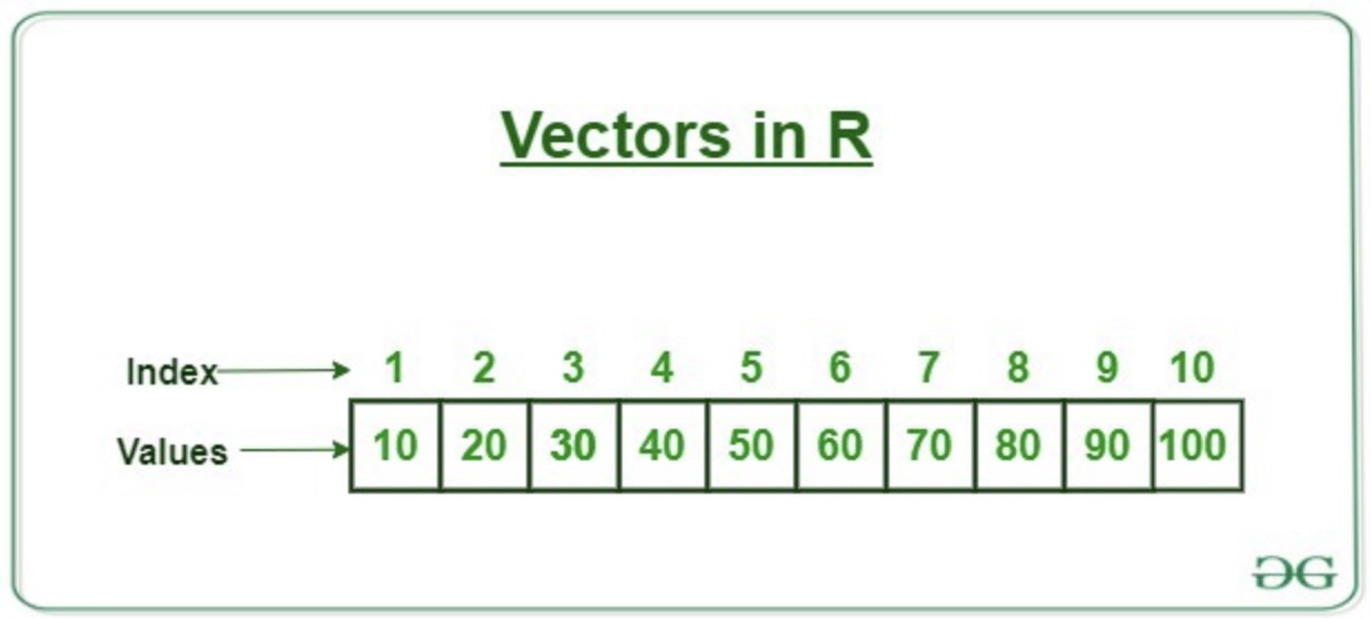
This example is a 1-dimensional vector that holds 10 values. You can see the values that we have saved are 10, 20, 30, 40, 50, 60, 70, 80, 90, and 100. The index tells us what position each value is in. The first value is at index 1, the second value is at index 2, and so on.

When creating a new vector, you want to make sure you are giving it a name that makes sense. For example, if you are creating a vector that holds the scores from a test, you might want to name it test_scores. This will help you remember what the vector is for when you are working with it later.

In order to create a vector, we can use the c() function. This function stands for “combine” and is used to combine multiple values into a single vector. For example, if we wanted to create a vector that holds the numbers from above, we could do it like this:

test_scores <- c(10, 20, 30, 40, 50, 60, 70, 80, 90, 100)

class(test_scores)

[1] "numeric"

Note : I used the class() function to check the type of the object. The output of this command is numeric. This tells us that the object is a numeric vector. This is because all of the values in the vector are numbers.

We can access the values by using the index. For example, if we wanted to access the first value in the vector, we could do it like this: test_scores[1]. This would return the value 10.

test_scores[1]

[1] 10

If I wanted to examine the 4th - 7th entries, I could do it like this: test_scores[4:7]. This would return the values 40, 50, 60, 70.

test_scores[4:7]

[1] 40 50 60 70

Note that we can’t just pick random locations in the vector. For example, if I wanted to print out the values in the 2nd, 5th, and 9th locations? The command test_scores[2, 5, 9] would not work. You would get an error message that stops your script.

Instead, we could create a vector that holds the locations we want to examine. For example, we could create a vector that holds the values 2, 5, 9 and use this vector in our command :

test_scores[c(2, 5, 9)]

[1] 20 50 90

You can also create a vector that holds text values. For example, you could create a vector that holds the names of the students in a class. This would look something like this:

student_names <- c("Alice", "Bob", "Charlie", "David", "Eve", "Frank", "Grace", "Hannah", "Ivy", "Jack")

class(student_names)

[1] "character"

Notice that this vector is of type character. This is because all of the values in the vector are text values. You can access the values in the same way as you would with a numeric vector. For example, if you wanted to access the first value in the vector, you could do it like this: student_names[1].

student_names[1]

[1] "Alice"

We have seen two examples. The first was a vector that contained numeric values and the second was a vector that contained text values. You can also create a vector that contains a mix of both. For example, you could create a vector that contains the names of the students in a class along with their test scores. This would look something like this:

student_data <- c("Alice", 100, "Bob", 90, "Charlie", 80, "David", 70, "Eve", 60, "Frank", 50, "Grace", 40, "Hannah", 30, "Ivy", 20, "Jack", 10)

When you create a vector that contains a mix of text and numeric values, you need to be careful.

When you create a vector that contains a mix of text and numeric values, R will convert the text values to a different type. For example, if you have a vector that contains both text and numeric values, the text values will be converted to a type called character. This is a type that is used to store text values. For example, if you have a vector that contains the values 10, 20, 30, "Alice", "Bob", the text values "Alice" and "Bob" will be converted to the type character. This is because R can’t store text values in a vector that is meant to hold numeric values.

class(student_data)

[1] "character"

If a vector contains text and numeric values, the text values will be converted to a different type. For example, if you have a vector that contains both text and numeric values, the text values will be converted to a type called character. This is a type that is used to store text values. For example, if you have a vector that contains the values 10, 20, 30, "Alice", "Bob", the text values "Alice" and "Bob" will be converted to the type character. This is because R can’t store text values in a vector that is meant to hold numeric values.

This can be problematic. For instance, what if we wanted to find the average of the test scores from the student_data vector? We would need to convert the text values to numeric values first. We can do this using the as.numeric() function. This function converts a vector to a numeric type. For example, if we wanted to convert the student_data vector to a numeric type, we could do it like this:

student_data <- as.numeric(student_data)

Warning: NAs introduced by coercion

student_data

 [1]  NA 100  NA  90  NA  80  NA  70  NA  60  NA  50  NA  40  NA  30  NA  20  NA
[20]  10

This is interesting because as we see the output, we get NA values. This is because the as.numeric() function can’t convert text values to numeric values. When it encounters a text value, it returns NA. This is a special value that is used to represent missing or undefined values. In this case, it is used to represent the text values that couldn’t be converted to numeric values.

So if we wanted to then find the average of the test scores, we could pull out the score sand save them into another vector. The test scores are in indices 2, 3, 6, 8, 10, 12, 14, 16, 18 and 20. We could save these into a new vector called test_scores2 and then find the average like this:

test_scores2 <- student_data[c(2, 4, 6, 8, 10, 12, 14, 16, 18, 20)]

Let’s check the vector to make sure it is correct :

test_scores2

 [1] 100  90  80  70  60  50  40  30  20  10

We can now find the average using the mean() function. This function calculates the average of a vector. For example, if we wanted to find the average of the test scores, we could do it like this:

mean(test_scores2)

[1] 55

The reason why a vector is not useful here is because it is trying to save two different forms of data at once. We are trying to save text and numeric data in the same vector. This is not a good idea. Surely there is an easier way to store the data! That is where data frames come in.

Data Frames

A data frame is a 2-dimensional (row and column) structure that can hold multiple elements. It is similar to a matrix, but it can hold different types of data in each column. For example, you could create a data frame that holds the names of the students in a class along with their test scores. This would look something like this:

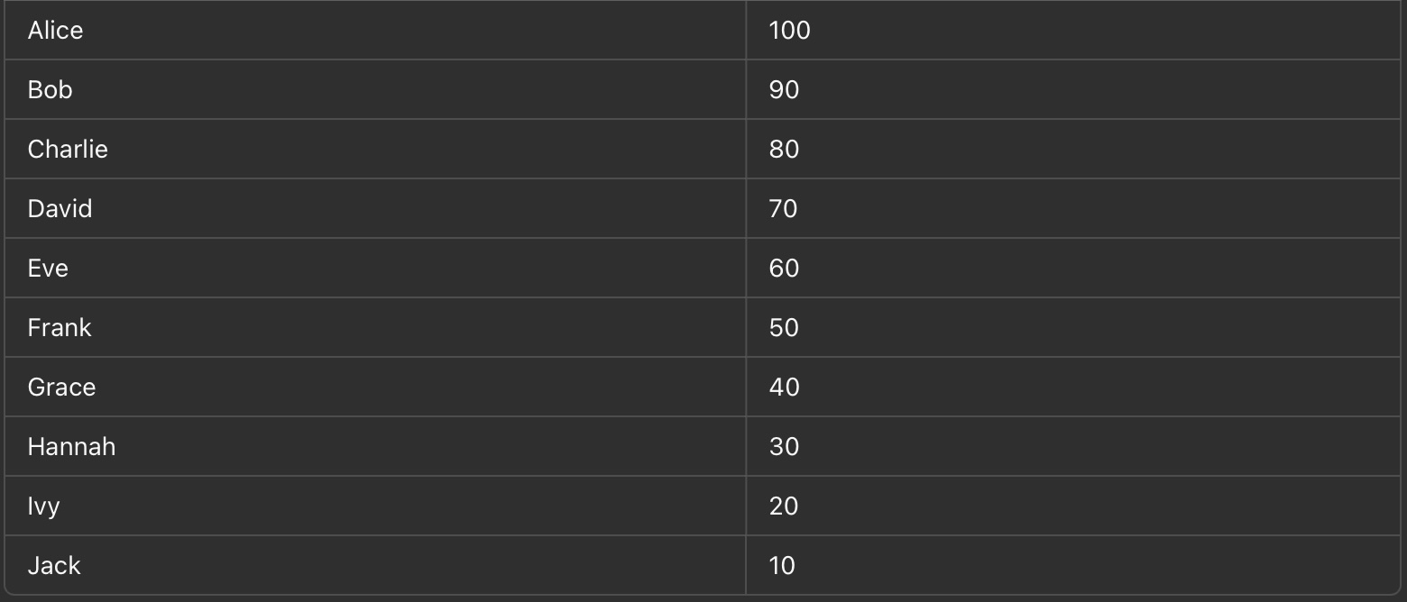
This example is a 2-dimensional data frame that holds 10 rows and 2 columns. This is an example of a data frame. In a data frame, each row is called an observation and each column is called a variable. This data frame has two variables: name and test_score. The name variable holds the names of the students in the class, while the test_score variable holds the test scores of the students.

When creating a new data frame, you want to make sure you are giving it a name that makes sense. For example, if you are creating a data frame that holds the names of the students in a class along with their test scores, you might want to name it student_data. This will help you remember what the data frame is for when you are working with it later.

In order to create a data frame, we can use the data.frame() function. This function is used to create a new data frame. For example, if we wanted to create a data frame that holds the names of the students in a class along with their test scores, we could do it like this:

student_data <- data.frame(
  name = c("Alice", "Bob", "Charlie", "David", "Eve", "Frank", "Grace", "Hannah", "Ivy", "Jack"),
  test_score = c(100, 90, 80, 70, 60, 50, 40, 30, 20, 10)
)

class(student_data)

[1] "data.frame"

In this example, we are creating a data one column at a time. Since we named these columns as name and test_score, we can access the values in the same way as we would with a vector. For example, if we wanted to access the first value in the name column, we could do it like this: student_data$name[1]. This would return the value Alice.

student_data$name[1]

[1] "Alice"

Similarly, if we wanted to access the first value in the test_score column, we could do it like this: student_data$test_score[1]. This would return the value 100.

student_data$test_score[1]

[1] 100

We could also the value in the fifth row and second column like this:

student_data[5, 2]

[1] 60

If we wanted to print out the entire first column, we could do it like this:

student_data$name

 [1] "Alice"   "Bob"     "Charlie" "David"   "Eve"     "Frank"   "Grace"  
 [8] "Hannah"  "Ivy"     "Jack"

If we wanted to print out the entire second column, we could do it like this:

student_data$test_score

 [1] 100  90  80  70  60  50  40  30  20  10

What happens if we wanted to print out the entore data frame? We could do it like this:

student_data

      name test_score
1    Alice        100
2      Bob         90
3  Charlie         80
4    David         70
5      Eve         60
6    Frank         50
7    Grace         40
8   Hannah         30
9      Ivy         20
10    Jack         10

These commands are nice, but if you have a large data set then just printing it off can be a bit overwhelming. We can use the head() function to print out the first few rows of the data frame. For example, if we wanted to print out the first 3 rows of the data frame, we could do it like this:

head(student_data, 3)

     name test_score
1   Alice        100
2     Bob         90
3 Charlie         80

If we wanted to print out the last few rows of the data frame, we could use the tail() function. For example, if we wanted to print out the last 5 rows

tail(student_data, 5)

     name test_score
6   Frank         50
7   Grace         40
8  Hannah         30
9     Ivy         20
10   Jack         10

The default amount of lines for head() and tail() is 6. If you don’t specify an amount of lines, it will print out 6 lines.

head(student_data)

     name test_score
1   Alice        100
2     Bob         90
3 Charlie         80
4   David         70
5     Eve         60
6   Frank         50

How is a data frame different from a tibble? Let’s talk about that next.

Tibbles

A tibble is a modern version of a data frame that is part of the tidyverse. It is similar to a data frame, but it has some additional features that make it easier to work with. For example, tibbles have a nicer print method that makes it easier to view the data. They also have some additional functions that make it easier to manipulate the data. For example, you can use the select() function to select specific columns from a tibble. You can also use the filter() function to filter rows based on a condition. These functions make it easier to work with tibbles than with data frames.

In order to create a tibble, we can use the tibble() function. This function is used to create a new tibble. For example, if we wanted to create a tibble that holds the names of the students in a class along with their test scores, we could do it like this:

# Make sure tidyverse is installed and loaded up. Remember, if you
# need to install it, use the following :

# install.packages(tidyverse)

# If it is already downloaded, then you just need to load up the library :

library(tidyverse)

Warning: package 'ggplot2' was built under R version 4.5.2

── Attaching core tidyverse packages ──────────────────────── tidyverse 2.0.0 ──
✔ forcats   1.0.0     ✔ readr     2.1.5
✔ ggplot2   4.0.1     ✔ stringr   1.6.0
✔ lubridate 1.9.4     ✔ tibble    3.3.0
✔ purrr     1.2.0     ✔ tidyr     1.3.1
── Conflicts ────────────────────────────────────────── tidyverse_conflicts() ──
✖ dplyr::filter() masks stats::filter()
✖ dplyr::lag()    masks stats::lag()
ℹ Use the conflicted package (<http://conflicted.r-lib.org/>) to force all conflicts to become errors

# I have already installed the tibble package, so I will just load it up

library(tibble)

student_data2 <- tibble(
  name = c("Alice", "Bob", "Charlie", "David", "Eve", "Frank", "Grace", "Hannah", "Ivy", "Jack"),
  test_score = c(100, 90, 80, 70, 60, 50, 40, 30, 20, 10)
)

class(student_data2)

[1] "tbl_df"     "tbl"        "data.frame"

In this example, we are creating a tibble that is similar to the data frame we created earlier. The main difference is that this tibble is part of the tidyverse. This means that it has some additional features that make it easier to work with. For example, we can use the select() function to select specific columns from the tibble. For example, if we wanted to select the name column from the tibble, we could do it like this:

select(student_data2, name)

# A tibble: 10 × 1
   name   
   <chr>  
 1 Alice  
 2 Bob    
 3 Charlie
 4 David  
 5 Eve    
 6 Frank  
 7 Grace  
 8 Hannah 
 9 Ivy    
10 Jack

If we wanted to select the test_score column from the tibble, we could do it like this:

select(student_data2, test_score)

# A tibble: 10 × 1
   test_score
        <dbl>
 1        100
 2         90
 3         80
 4         70
 5         60
 6         50
 7         40
 8         30
 9         20
10         10

If I want all of the students that got higher than a 65 for their test score, I could use the filter() command to help us out. The filter() command needs two arguments. The first is the name of the tibble and the second is the condition that we want to filter on. For example, if we wanted to filter out all of the students that got higher than a 65 on their test, we could do it like this:

filter(student_data2, test_score > 65)

# A tibble: 4 × 2
  name    test_score
  <chr>        <dbl>
1 Alice          100
2 Bob             90
3 Charlie         80
4 David           70

Another advantage a tibble has over a data frame is that it is easier to work with when you are working with large data sets. For example, if you have a data set that has 1 million rows, it can be difficult to work with a data frame. This is because data frames are stored in memory, and if you have a large data set, it can take up a lot of memory. This can slow down your computer and make it difficult to work with the data. Tibbles are designed to be more memory efficient than data frames. This means that they can handle larger data sets more easily. This makes it easier to work with large data sets in R.

Conclusion

In conclusion, vectors, data frames, and tibbles are all useful structures that can be used to store data. Vectors are 1-dimensional structures that can hold multiple elements. Data frames are 2-dimensional structures that can hold multiple elements. Tibbles are a modern version of data frames that are part of the tidyverse. They have some additional features that make them easier to work with. All of these structures are useful for storing data in R, and you will likely use all of them at some point when working with data in R.

Practice Problems

In this part of the assignment, you will practice creating different types of vectors in R and using common commands associated with them, such as determining their class. Each problem will involve creating a unique type of vector and performing specific operations.

Problem 1: Numeric Vector

Task: Create a numeric vector containing the first 10 positive integers and determine its class.

Steps:

Create a numeric vector called num_vector containing the numbers 1 to 10.
Determine the class of num_vector and save the result to the variable class_num_vector.
Check your work.

Solution


# Create numeric vector
num_vector <- c(1, 2, 3, 4, 5, 6, 7, 8, 9, 10)

# or

num_vector <- c(1:10)


# Determine the class of num_vector
class_num_vector <- class(num_vector)

num_vector
class_num_vector

Problem 2: Character Vector

Task: Create a character vector containing the names of the first five months of the year and determine its class.

Steps:

Create a character vector char_vector containing the names “January”, “February”, “March”, “April”, and “May”.
Determine the class of char_vector and save the result to the variable class_char_vector.
Check your work.

Solution


# Create character vector
char_vector <- c("January", "February", "March", "April", "May")

# Determine the class of the vector
class_char_vector <- class(char_vector)

# Check your work 

char_vector
class_char_vector

Problem 3: Logical Vector

Task: Create a logical vector containing alternating TRUE and FALSE values for a length of 8 and determine its class.

Steps:

Create a logical vector log_vector with 8 terms alternating TRUE and FALSE values.
Determine the class of the vector and save the result to the variable class_log_vector.
Check your work.

Solution


# Create logical vector
log_vector <- c(TRUE, FALSE, TRUE, FALSE, TRUE, FALSE, TRUE, FALSE)

# Determine the class of the vector
class_log_vector <- class(log_vector)

# Check your work

log_vector

class_log_vector

Problem 4: Factor Vector

Task: Create a factor vector from a character vector containing three levels: “High”, “Medium”, and “Low”, and determine its class.

Steps:

Create a character vector char_levels with the 5 values “High”, “Medium”, “Low”, “High”, “Low”.
Using the factor command, convert this character vector into a factor vector called fact_vector with levels “Low”, “Medium” and “High”.
Determine the class of the factor vector fact_vector and save the result to the variable class_fact_vector.
Check your work.

Solution


# Create character vector with levels

char_levels <- c("High", "Medium", "Low", "High", "Low")

# Convert to factor vector

fact_vector <- factor(char_levels, levels = c("Low", "Medium", "High"))

# Determine the class of the factor vector

class_fact_vector <- class(fact_vector)

# Check your work

fact_vector

class_fact_vector

Problem 5: Complex Vector

Task: Create a complex vector containing the first four complex numbers with real and imaginary parts, and determine its class.

Steps:

Create a complex vector comp_vector with values 1+2i, 3+4i, 5+6i, 7+8i.
Determine the class of the vector and save the result to the variable class_comp_vector.
Check your work.

Solution


# Create complex vector

comp_vector <- c(1+2i, 3+4i, 5+6i, 7+8i)

# Determine the class of the vector

class_comp_vector <- class(comp_vector)

# Check your work

comp_vector

class_comp_vector

In this part of the assignment, you will practice creating different types of data frames in R and using common commands associated with them, such as pulling out values, and using head() and tail() functions. Each problem will involve creating a unique type of data frame and performing specific operations.

Problem 6: Creating a Data Frame for Students’ Scores

Task: Create a data frame containing the names and scores of five students in a math test. Use commands to pull out specific values and display the first few rows of the data frame.

Steps:

Create a data frame students_df with columns Name and Score. Use the following:
- Name: “Alice”, “Bob”, “Charlie”, “David”, “Eve”
- Score: 85, 90, 78, 92, 88
Create a variable called alice_score where you pull out the score of the student named “Alice”.
Save the first three rows of students_df into the variable ’head_students_df`
Check your work

Solution


# Create data frame

students_df <- data.frame(
  Name = c("Alice", "Bob", "Charlie", "David", "Eve"),
  Score = c(85, 90, 78, 92, 88)
)

# Pull out the score of Alice

alice_score <- students_df$Score[students_df$Name == "Alice"]

# Display the first three rows of the data frame

head_students_df <- head(students_df, 3)

# Check your work

students_df

alice_score

head_students_df

Problem 7: Creating a Data Frame for Monthly Expenses

Task: Create a data frame containing the monthly expenses for three categories (Rent, Food, Utilities) over six months. Use commands to pull out specific values and display the last few rows of the data frame.

Steps:

Create a data frame expenses_df with columns Month, Rent, Food, and Utilities.
- Month: “January”, “February”, “March”, “April”, “May”, “June”
- Rent: 1000, 1000, 1000, 1000, 1000, 1000
- Food: 300, 320, 310, 330, 340, 350
- Utilities: 150, 160, 155, 165, 170, 175
Pull out the food expense for the month of March and place it in the variable march_food_expense.
Display the last two rows of the data frame using tail() and save it to the variable tail_expenses_df.
Check your work.

Solution


# Create data frame

expenses_df <- data.frame(
  Month = c("January", "February", "March", "April", "May", "June"),
  Rent = c(1000, 1000, 1000, 1000, 1000, 1000),
  Food = c(300, 320, 310, 330, 340, 350),
  Utilities = c(150, 160, 155, 165, 170, 175)
)

# Pull out the food expense for March

march_food_expense <- expenses_df$Food[expenses_df$Month == "March"]

# Display the last two rows of the data frame

tail_expenses_df <- tail(expenses_df, 2)

# Check your work

expenses_df

march_food_expense

tail_expenses_df

Problem 8: Creating a Data Frame for Employee Information

Task: Create a data frame containing the employee information (ID, Name, Department, Salary). Use commands to pull out specific values and display the first few rows of the data frame.

Steps:

Create a data frame employee_df with columns ID, Name, Department, and Salary.
- ID: 1001, 1002, 1003, 1004, 1005
- Name: “John”, “Jane”, “Doe”, “Smith”, “Emily”
- Department: “HR”, “Finance”, “IT”, “Marketing”, “Admin”
- Salary: 50000, 60000, 55000, 70000, 65000
Pull out the department of the employee with ID 1003 and save it to the variable dept_id_1003.
Display the first four rows of the data frame using head() and save it to the variable head_employee_df.
Check your work.

Solution


# Create data frame

employee_df <- data.frame(
  ID = c(1001, 1002, 1003, 1004, 1005),
  Name = c("John", "Jane", "Doe", "Smith", "Emily"),
  Department = c("HR", "Finance", "IT", "Marketing", "Admin"),
  Salary = c(50000, 60000, 55000, 70000, 65000)
)

# Pull out the department of the employee with ID 1003

dept_id_3 <- employee_df$Department[employee_df$ID == 1003]

# Display the first four rows of the data frame

head_employee_df <- head(employee_df, 4)

# Check your work

employee_df

dept_id_3

head_employee_df

Problem 9: Creating a Data Frame for Product Sales

Task: Create a data frame containing the product sales information (ProductID, ProductName, UnitsSold, Revenue). Use commands to pull out specific values and display the last few rows of the data frame.

Steps:

Create a data frame sales_df with columns ProductID, ProductName, UnitsSold, and Revenue.
- ProductID: 101, 102, 103, 104, 105
- ProductName: “Laptop”, “Tablet”, “Smartphone”, “Desktop”, “Monitor”
- UnitsSold: 50, 100, 200, 30, 80
- Revenue: 50000, 30000, 40000, 15000, 20000
Pull out the revenue of the product named “Tablet” and save it to the variable tablet_revenue.
Display the last three rows of the data frame using tail() and save it to the variable tail_sales_df.
Check your work.

Solution


# Create data frame
sales_df <- data.frame(
  ProductID = c(101, 102, 103, 104, 105),
  ProductName = c("Laptop", "Tablet", "Smartphone", "Desktop", "Monitor"),
  UnitsSold = c(50, 100, 200, 30, 80),
  Revenue = c(50000, 30000, 40000, 15000, 20000)
)

# Pull out the revenue of the product named Tablet
tablet_revenue <- sales_df$Revenue[sales_df$ProductName == "Tablet"]

# Display the last three rows of the data frame
tail_sales_df <- tail(sales_df, 3)

# Check your work

sales_df

tablet_revenue

tail_sales_df

Problem 10: Creating a Data Frame for Weather Data

Task: Create a data frame containing the weather data (Day, Temperature, Humidity, WindSpeed). Use commands to pull out specific values and display the first and last few rows of the data frame.

Steps:

Create a data frame weather_df with columns Day, Temperature, Humidity, and WindSpeed.
- Day: 1 to 10
- Temperature: 25, 27, 24, 26, 28, 29, 30, 31, 32, 33
- Humidity: 80, 82, 78, 76, 79, 81, 83, 85, 84, 86
- WindSpeed: 10, 12, 11, 13, 14, 15, 16, 17, 18, 19
Pull out the temperature on the 5th day and save it to the variable temp_day_5.
Display the first two and last two rows of the data frame using head() and tail() and save them to the variables head_weather_df and tail_weather_df.
Check your work.

Solution


# Create data frame

weather_df <- data.frame(
  Day = 1:10,
  Temperature = c(25, 27, 24, 26, 28, 29, 30, 31, 32, 33),
  Humidity = c(80, 82, 78, 76, 79, 81, 83, 85, 84, 86),
  WindSpeed = c(10, 12, 11, 13, 14, 15, 16, 17, 18, 19)
)

# Pull out the temperature on the 5th day

temp_day_5 <- weather_df$Temperature[weather_df$Day == 5]

# Display the first two rows of the data frame

head_weather_df <- head(weather_df, 2)

# Display the last two rows of the data frame

tail_weather_df <- tail(weather_df, 2)

# Check your work

weather_df

temp_day_5

head_weather_df

tail_weather_df

In this part of the assignment, you will practice creating different types of tibbles in R and using common commands associated with them, such as creating a tibble, converting a data frame to a tibble, selecting columns, and filtering rows. Each problem will involve creating or manipulating tibbles and performing specific operations.

Problem 11: Creating a Tibble for Students’ Scores

Task: Create a tibble containing the names and scores of five students in a math test. Use commands to select specific columns and display the tibble.

Steps:

Create a tibble students_tbl with columns Name and Score.
- Name: “Alice”, “Bob”, “Charlie”, “David”, “Eve”
- Score: 85, 90, 78, 92, 88
Select the Name column from the tibble and save it to the variable name_column.
Display the entire tibble students_tbl and the selected column name_column.
Check your work.

Solution

# Load the tibble package, if needed
# library(tibble)

# Create tibble

students_tbl <- tibble(
  Name = c("Alice", "Bob", "Charlie", "David", "Eve"),
  Score = c(85, 90, 78, 92, 88)
)

# Select the Name column

name_column <- select(students_tbl, Name)

# Display the tibble

students_tbl

# Display the name column

name_column

Problem 12: Converting a Data Frame to a Tibble for Monthly Expenses

Task: Create a data frame containing the monthly expenses for three categories (Rent, Food, Utilities) over six months and convert it to a tibble. Use commands to filter specific rows and display the tibble.

Steps:

Create a data frame expenses_df with columns Month, Rent, Food, and Utilities.
- Month: “January”, “February”, “March”, “April”, “May”, “June”
- Rent: 1000, 1000, 1000, 1000, 1000, 1000
- Food: 300, 320, 310, 330, 340, 350
- Utilities: 150, 160, 155, 165, 170, 175
Convert the data frame to a tibble expenses_tbl.
Filter the tibble to include only the rows where Rent is greater than 1000 and save it to the variable filtered_expenses_tbl.
Display both tibbles.

Solution

# Create data frame

expenses_df <- data.frame(
  Month = c("January", "February", "March", "April", "May", "June"),
  Rent = c(1000, 1000, 1000, 1000, 1000, 1000),
  Food = c(300, 320, 310, 330, 340, 350),
  Utilities = c(150, 160, 155, 165, 170, 175)
)

# Convert data frame to tibble

expenses_tbl <- as_tibble(expenses_df)

# Filter the tibble

filtered_expenses_tbl <- filter(expenses_tbl, Rent > 1000)

# Display the tibbles

expenses_tbl

filtered_expenses_tbl

Problem 13: Creating a Tibble for Employee Information and Selecting Columns

Task: Create a tibble containing the employee information (ID, Name, Department, Salary). Use commands to select specific columns and display the tibble.

Steps:

Create a tibble employee_tbl with columns ID, Name, Department, and Salary.
- ID: 1, 2, 3, 4, 5
- Name: “John”, “Jane”, “Doe”, “Smith”, “Emily”
- Department: “HR”, “Finance”, “IT”, “Marketing”, “Admin”
- Salary: 50000, 60000, 55000, 70000, 65000
Select the Name and Salary columns from the tibble.
Display both tibbles.

Solution

# Load the tibble package, if needed
# library(tibble)

# Create tibble

employee_tbl <- tibble(
  ID = c(1, 2, 3, 4, 5),
  Name = c("John", "Jane", "Doe", "Smith", "Emily"),
  Department = c("HR", "Finance", "IT", "Marketing", "Admin"),
  Salary = c(50000, 60000, 55000, 70000, 65000)
)

# Select the Name and Salary columns

name_salary_columns <- select(employee_tbl, Name, Salary)

# Display the tibble

employee_tbl

name_salary_columns

Problem 14: Creating a Tibble for Product Sales and Filtering Rows

Task: Create a tibble containing the product sales information (ProductID, ProductName, UnitsSold, Revenue). Use commands to filter specific rows and display the tibble.

Steps:

Create a tibble sales_tbl with columns ProductID, ProductName, UnitsSold, and Revenue.
- ProductID: 101, 102, 103, 104, 105
- ProductName: “Laptop”, “Tablet”, “Smartphone”, “Desktop”, “Monitor”
- UnitsSold: 50, 100, 200, 30, 80
- Revenue: 50000, 30000, 40000, 15000, 20000
Filter the tibble to include only the rows where UnitsSold is greater than 50 and save it to the variable filtered_sales_tbl.
Display the entire tibble sales_tbl and the filtered tibble filtered_sales_tbl.

Solution

# Create tibble

sales_tbl <- tibble(
  ProductID = c(101, 102, 103, 104, 105),
  ProductName = c("Laptop", "Tablet", "Smartphone", "Desktop", "Monitor"),
  UnitsSold = c(50, 100, 200, 30, 80),
  Revenue = c(50000, 30000, 40000, 15000, 20000)
)

# Filter the tibble

filtered_sales_tbl <- filter(sales_tbl, UnitsSold > 50)

# Display the tibble

sales_tbl

filtered_sales_tbl

Problem 15: Creating a Tibble for Weather Data and Using `head()` and `tail()`

Task: Create a tibble containing the weather data (Day, Temperature, Humidity, WindSpeed). Use commands to display the first and last few rows of the tibble.

Steps:

Create a tibble weather_tbl with columns Day, Temperature, Humidity, and WindSpeed.
- Day: 1 to 10
- Temperature: 25, 27, 24, 26, 28, 29, 30, 31, 32, 33
- Humidity: 80, 82, 78, 76, 79, 81, 83, 85, 84, 86
- WindSpeed: 10, 12, 11, 13, 14, 15, 16, 17, 18, 19
Display the first three rows of the tibble using head() and save it to the variable head_weather_tbl.
Display the last three rows of the tibble using tail() and save it to the variable tail_weather_tbl.
Check your work.

Solution

# Create tibble

weather_tbl <- tibble(
  Day = 1:10,
  Temperature = c(25, 27, 24, 26, 28, 29, 30, 31, 32, 33),
  Humidity = c(80, 82, 78, 76, 79, 81, 83, 85, 84, 86),
  WindSpeed = c(10, 12, 11, 13, 14, 15, 16, 17, 18, 19)
)

# Display the first three rows of the tibble

head_weather_tbl <- head(weather_tbl, 3)

# Display the last three rows of the tibble

tail_weather_tbl <- tail(weather_tbl, 3)

weather_tbl

head_weather_tbl

tail_weather_tbl

Problem 16: Finding the Number of Rows in a Data Frame

Task: Install the database Star Wars data set and load it into a data frame called starwars_DF. Use commands to find the number of rows in the data frame.

Steps:

Install the Star Wars database package and load it into a data frame called starwars_DF.
Use two different methods for finding the number of rows in your data frame. What does this represent?

Solution


# The number of rows in the data frame represents the number of observations 
# or records in the dataset.

# You can use the nrow() function to find the number of rows in the data frame.

nrow(starwars_DF)

# You can also use the dim() function to find the number of rows and columns 
# in the data frame.

dim(starwars_DF)

Problem 17: Finding the Number of Columns in a Data Frame

Task: Using starwars_DF, find the number of columns in the data frame.

Solution


# You can use the `dim()` function to find the number of rows and columns in a data frame.

dim(starwars_DF)

# You can use the `ncol()` function to find the number of columns in a data frame.

ncol(starwars_DF)

Problem 18: Finding the Variable Names in a Data Frame

Task: Using starwars_DF, find the variable names in the data frame. Use the names() and colnames() commands to list off the variable names in the data frame?

Solution

# names() can be used to list off the variable names in a data frame.

names(starwars_DF)

# colnames() can also be used to list off the variable names in a data frame.

colnames(starwars_DF)

Problem 19: Pulling Out a Variable in a Data Frame

Task: Using starwars_DF, pull out the “height” variable and save it to a new variable called SW_height. Use three different methods to do this. How many values are listed? Does this raise any concerns?

Steps:

Use the $ operator to pull out the “height” variable and save it to SW_height.
Use the [,] operator to pull out the “height” variable and save it to SW_height_2.
Use the [[ ]] operator to pull out the “height” variable and save it to SW_height_3.
Check the length of SW_height to see how many values are listed.

How many values are listed? Does this raise any concerns?

Solution

# We want to pull out the "height" variable. Carry out two different commands that will pull out this information and save it to a new variable called SW_height. How many values are listed? Does this raise any concerns?

SW_height <- starwars_DF$height

SW_height_2 <- starwars_DF[,2]

SW_height_3 <- starwars_DF[["height"]]

length(SW_height)

Problem 20: Checking the New Variable

Task: Check the new variable SW_height to see if there might be any errors in the data.

** Steps:**

Print out the new variable SW_height to see if there are any errors in the data.
Do all of the observations have a value for height? If not, how many are missing and who are they missing from? We can use the is.na() function to check for missing values.
Print out the number of missing values in the height variable using the sum() function.

Solution

# Check the new variable SW_height to see if there might be any errors in the data.

print(SW_height)

# Check if there are any missing values in the height variable

missing_values <- is.na(SW_height)

# Print out the number of missing values in the height variable

missing_count <- sum(missing_values)

print(missing_count)

Problem 21 : Printing Out the Heights from Smallest to Largest

Task: Using SW_height, print out the heights from smallest to largest. Also save the sorted list to a new variable called SW_height_sorted_1.

Steps:

Use the sort() function to sort the heights from smallest to largest and save it to SW_height_sorted_1.
Print out the sorted heights.

Solution

# Print out the heights from smallest to largest

SW_height_sorted_1 <- sort(SW_height)

# Check your work

print(SW_height_sorted_1)

Problem 22 : Printing Out the Heights from Largest to Smallest

Task: Using SW_height, print out the heights from largest to smallest. Also save the sorted list to a new variable called SW_height_sorted_2.

Steps:

Use the sort help file to see how to sort the values from largest to smallest.
Print out the heights from largest to smallest and save new sorted list to SW_height_sorted_2

Solution

# Print out the heights from largest to smallest

SW_height_sorted_2 <- sort(SW_height, decreasing = TRUE)

# Check your work

print(SW_height_sorted_2)

Problem 23 : Find The Maximum Value

Task: Using SW_height, find the maximum value of the height variable. Use two different methods to do this and save the value to a new variable called SW_max_height and SW_max_height_2.

Steps:

Use the max() function to find the maximum value of the height variable and save it to SW_max_height.
Use the sort() function to sort the data where the maximum value is first and save the sorted list to SW_max_height_sorted. The largest value should be the first value in the sorted list. Save that value to SW_max_height_2.

Vectors

Data Frames

Tibbles

Conclusion

Practice Problems

Problem 1: Numeric Vector

Problem 2: Character Vector

Problem 3: Logical Vector

Problem 4: Factor Vector

Problem 5: Complex Vector

Problem 6: Creating a Data Frame for Students’ Scores

Problem 7: Creating a Data Frame for Monthly Expenses

Problem 8: Creating a Data Frame for Employee Information

Problem 9: Creating a Data Frame for Product Sales

Problem 10: Creating a Data Frame for Weather Data

Problem 11: Creating a Tibble for Students’ Scores

Problem 12: Converting a Data Frame to a Tibble for Monthly Expenses

Problem 13: Creating a Tibble for Employee Information and Selecting Columns

Problem 14: Creating a Tibble for Product Sales and Filtering Rows

Problem 15: Creating a Tibble for Weather Data and Using head() and tail()

Problem 16: Finding the Number of Rows in a Data Frame

Problem 17: Finding the Number of Columns in a Data Frame

Problem 18: Finding the Variable Names in a Data Frame

Problem 19: Pulling Out a Variable in a Data Frame

Problem 20: Checking the New Variable

Problem 21 : Printing Out the Heights from Smallest to Largest

Problem 22 : Printing Out the Heights from Largest to Smallest

Problem 23 : Find The Maximum Value

Problem 15: Creating a Tibble for Weather Data and Using `head()` and `tail()`