Statistics Language

As we start to consider analyzing data, we need to be able to communicate with other data scientists. This is where statistics language comes in. We want to take some time to define some terms that we will be using throughout the course. For now we will just focus on foundational terms. As we develop different analytic skills, we will introduce more terms.

Population

The population is the entire group that we are interested in studying. For example, if we are interested in studying the average height of all people in the United States, then the population would be all people in the United States.

Parameter

A parameter is a number that describes a population. For example, the average height of all people in the United States is a parameter. Two of the more common parameters are the mean and the standard deviation. These are used to describe the central tendency and the spread of a population. The mean is typically denoted by the Greek letter mu (μ) and the standard deviation is typically denoted by the Greek letter sigma (σ). We will briefly talk about these measures below and go into more detail in later sections.

Many studies that are done are ones that are trying to estimate a parameter. Unfortunately, there is only one way to know the true value of a parameter and that is to measure the entire population. This is not feasible in most cases as the amount of time and resources to contact every member of a population is not practical. We can, however, take what is called a sample of the population and use that to estimate the parameter.

Sample

A sample is a subset of the population. For example, if we are interested in studying the average height of all people in the United States, then a sample could be a group of 100 people from the United States. This is a much easier way to get information about the population rather than having to contact every member of the population.

There are several different methods one can use to take a sample. We will discuss these methods in later sections.

Statistic

A statistic is a number that describes a sample. For example, the average height of a group of 100 people from the United States is a statistic. Two of the more common statistics are the sample mean and the sample standard deviation. These are used to describe the central tendency and the spread of a sample. The sample mean is typically denoted by the letter x-bar (x̄) and the sample standard deviation is typically denoted by the letter s.

If we are trying to answer a question about the population, for instance the average height of all people in the United States, we can take a sample of the population and use the value from the sample as an estimate for the parameter from the population. This is the basis of inferential statistics, which we mention next.

Inferential Statistics

Inferential statistics are used to make inferences from a sample to a population. In other words, inferential statistics are used to make predictions about a population based on a sample. The following graphic demonstrates the process.

We are wanting to determine a population parameter μ
We take a sample from the population
Calculate the value of the statistic x̄ from the sample.
Use the sample statistic x to estimate the population parameter μ.

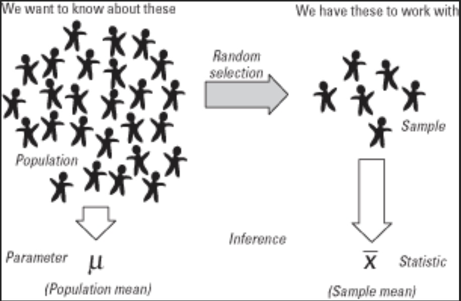
This process is the basis of inferential statistics. Using the sample to help us determine estimates of the population parameter.

Descriptive Statistics

Descriptive statistics are used to describe the basic features of the data in a study. They provide simple summaries about the sample and the measures. For our purposes we will focus on measures of central tendency (mean, median, mode) and measures of spread (standard deviation, variance, 5-Number summary). We will discuss these in more detail in later sections.

Confidence Interval

We are using a sample to estimate a population parameter. Unfortunately, if we were to take multiple samples from the population, we would get different values for the parameter. This is because the sample is only a portion of the population. The sample you take the first time is almost assuredly going to be different from the sample you take the second time. This means that the statistic from the first sample is going to be different from the statistic from the second sample.

This is the reason why we will estimate a parameter with a confidence interval. A confidence interval is a range of values that is likely to contain the true value of a parameter. For example, a 95% confidence interval for the average height of all people in the United States would be a range of values that is likely to contain the true average height with 95% confidence. The confidence interval is based on the sample statistic and a margin of error. The higher the confidence level, the wider the confidence interval. We will discuss confidence intervals in more detail in later sections.

Distribution

The distribution of a data set tells us two things : the values in the data set and how often they occur.

Here is an example of a distribution of the number of times a person goes to the gym in a week.

# We need the tibble function, so load up the tidyverse package

library(tidyverse)

Warning: package 'ggplot2' was built under R version 4.5.2

# Create a data frame

df <- tibble(
  gym_visits = c(0, 1, 2, 3, 4, 5, 6, 7),
  frequency = c(10, 20, 30, 40, 50, 40, 30, 20)
)

df

# A tibble: 8 × 2
  gym_visits frequency
       <dbl>     <dbl>
1          0        10
2          1        20
3          2        30
4          3        40
5          4        50
6          5        40
7          6        30
8          7        20

In this example, the distribution tells us how many times a person goes to the gym in a week and how often that occurs. For example, 40 people go to the gym 3 times a week or 30 people go to the gym 6 times a week.

Outlier

An outlier is a data point that is significantly different from the other data points in a dataset. Outliers can have a significant impact on the results of statistical analyses, especially for means and standard deviations. Outliers can be caused by errors in data collection, measurement error, or natural variation in the data.

In the following example, if someone went to the gym 15 times in a week would be considered an outlier. This is because the number of times a person goes to the gym in a week is typically between 0 and 7.

Depending on the data set, outliers could occur in either the high or the low direction.

Normal Distribution

One of the more typical distributions one will work with is the normal distribution. A normal distribution is a symmetric unimodal distributionin which the values are distributed around the mean according to a bell-shaped curve. The normal distribution is characterized by its mean and standard deviation. In other words, the mean and standard deviation determine the shape of the normal distribution. The mean determines the center of the distribution and the standard deviation determines the height and width of the distribution.

Skewness

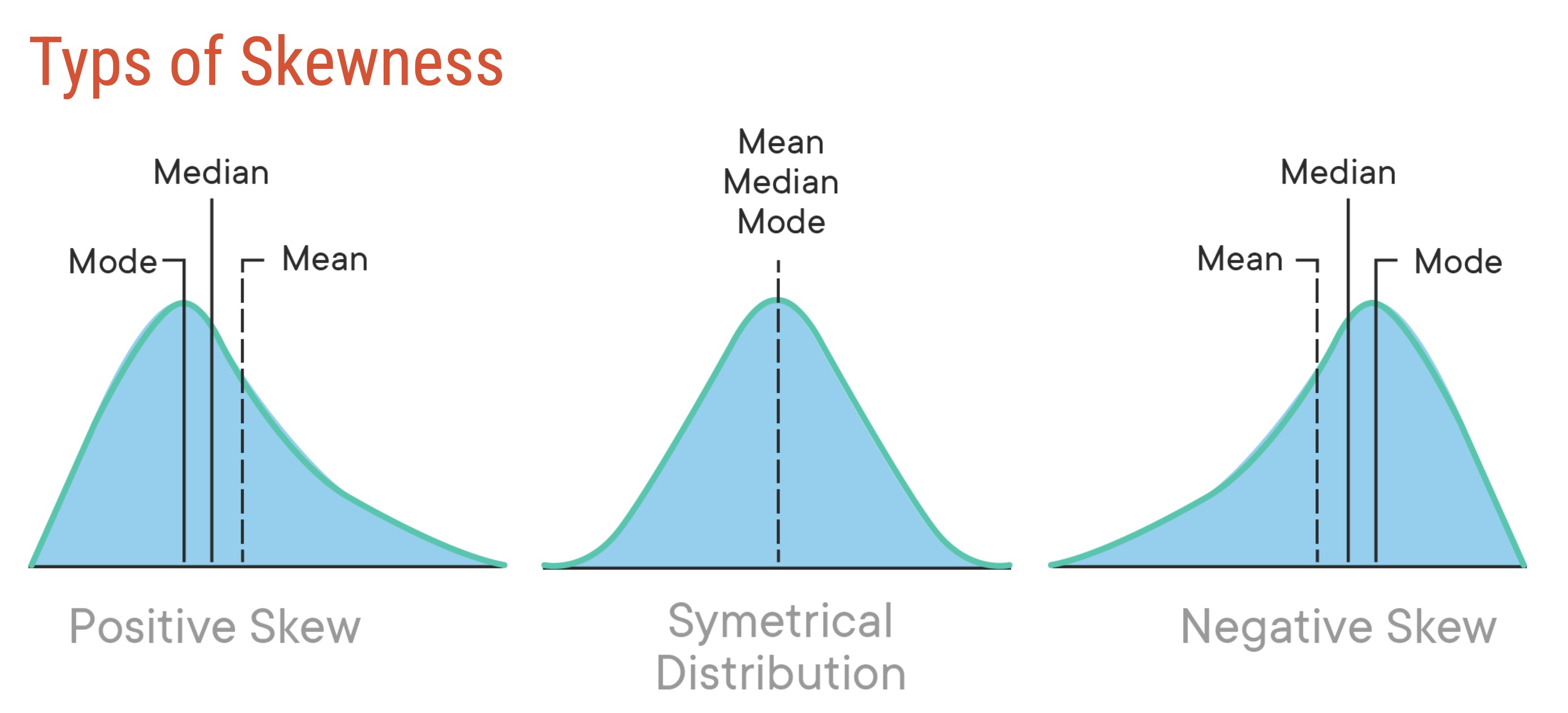
Once we know the distribution of a data set, we will often draw a picture of the distribution. One of the descriptors we will look for is skewness. Skewness is a measure of the asymmetry of a distribution. A distribution is symmetric if the left and right sides are mirror images of each other. A distribution is positively skewed (or skewed to the right)
if the right tail is longer than the left tail, and negatively skewed (or skewed left) if the left tail is longer than the right tail.

Here is a graphic giving examples of each type of skewness.