# Here are some typical packages we have been using. You may not need all of them,
# but we will load them anyway just in case.

library(tidyverse)
library(dplyr)
library(knitr)
library(gt)
library(janitor)Create A Table Challenge 1
Evan Miyakawa has a doctorate in Statistics and he uses his skills to analyze several sports, including college basketball. He hosts a website that shows his work with several links to articles, blogs, interviews, etc., related to men’s college basketball.
On Dec 19, 2026 he posted a table that showed the top 10 teams, along with their Offensive Rating (O-Rate), Defensive Rating (D-Rate), and Net Rating (Net Rate). The table is shown below:
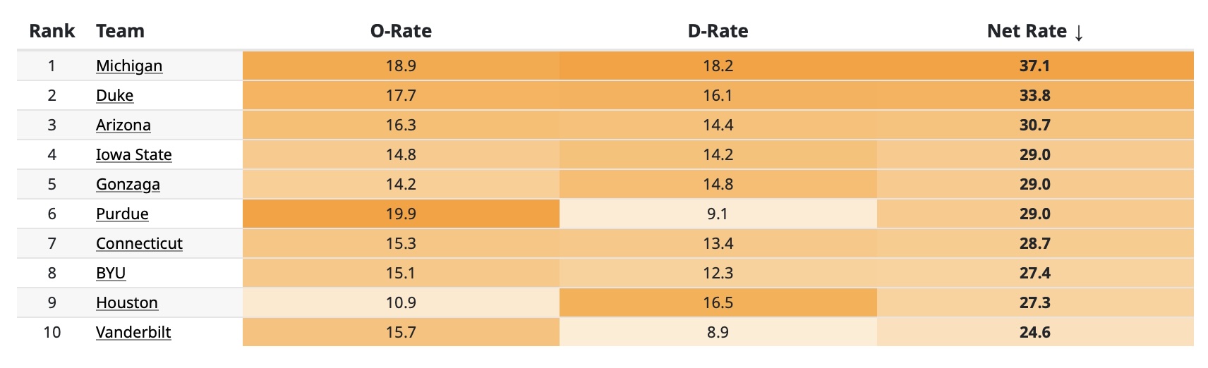
Your challenge is to recreate this table as best as you can using the skills we have developed so far.
Step 0 : Load the libraries you will need.
Step 1 : Create the data frame.
We are not going to do anything fancy here. Just create a data frame with the data shown in the table above and store the result in the variable rankings.
# Your code here : Create each column one at a time.

rankings <- data.frame(
  Rank = __ : __,
  Team = c("______", "______", "______", "______", "______",
           "______", "______", "______", "______", "______"),
  O_Rate = c(_____, _____, _____, _____, _____,
             _____, _____, _____, _____, _____),
  D_Rate = c(_____, _____, _____, _____, _____,
             _____, _____, _____, _____, _____),
  Net_Rate = c(_____, _____, _____, _____, _____,
               _____, _____, _____, _____, _____)
)
# Print the data frame to verify

rankings
Solution
rankings <- data.frame(
  Rank = 1:10,
  Team = c("Michigan", "Duke", "Arizona", "Iowa State", "Gonzaga",
           "Purdue", "Connecticut", "BYU", "Houston", "Vanderbilt"),
  O_Rate = c(18.9, 17.7, 16.3, 14.8, 14.2,
             19.9, 15.3, 15.1, 10.9, 15.7),
  D_Rate = c(18.2, 16.1, 14.4, 14.2, 14.8,
             9.1, 13.4, 12.3, 16.5, 8.9),
  Net_Rate = c(37.1, 33.8, 30.7, 29.0, 29.0,
               29.0, 28.7, 27.4, 27.3, 24.6)
)

# Print the data frame to verify

rankings
Rank Team O_Rate D_Rate Net_Rate
1 1 Michigan 18.9 18.2 37.1
2 2 Duke 17.7 16.1 33.8
3 3 Arizona 16.3 14.4 30.7
4 4 Iowa State 14.8 14.2 29.0
5 5 Gonzaga 14.2 14.8 29.0
6 6 Purdue 19.9 9.1 29.0
7 7 Connecticut 15.3 13.4 28.7
8 8 BYU 15.1 12.3 27.4
9 9 Houston 10.9 16.5 27.3
10 10 Vanderbilt 15.7 8.9 24.6Step 2 : Create a basic table using the gt( ) package.
For the first step, just create a basic table using the gt package and store the result in the variable rankings_table. We can start using these conventions:
- Use
data_color()to color the cells in the O_Rate, D_Rate, and Net_Rate columns. - Use a color palette that goes from white to orange.
- Set the domain to NULL so that the colors are scaled automatically to the data range.
# Your code here : List the columns that are going to get colors,
# and the colors to use.

rankings_table <- rankings %>%
  gt() %>%
  data_color(
    columns = c(_______, _______, _______),      # List the columns to color
    fn = scales::col_numeric(
      palette = c("_______", "_______"), # Gradient from white to orange
      domain = NULL                     # Automatically scales to the data range
    )
  )

# Display the table
rankings_table %>% as_raw_html()
Note 1 : The fn argument in the data_color( ) function is used to specify a function that generates colors based on the data values in the specified columns.
Note 2 : The scales::col_numeric( ) is a function provided by the scales package in R. We could have loaded the scales package separately, and just used col_numeric( ).
It creates a mapping between numeric values and a pre-defined color gradient (e.g., from “white” to “orange”). It is used for interpolating colors across a numeric range (domain) for visualization purposes.
Solution
rankings_table <- rankings %>%
  gt() %>%
  data_color(
    columns = c(O_Rate, D_Rate, Net_Rate),    # List the columns to color
    fn = scales::col_numeric(
      palette = c("white", "orange"),   # Gradient from white to orange
      domain = NULL                     # Automatically scales to the data range
    )
  )

# Display the table
rankings_table| Rank | Team | O_Rate | D_Rate | Net_Rate |
|---|---|---|---|---|
| 1 | Michigan | 18.9 | 18.2 | 37.1 |
| 2 | Duke | 17.7 | 16.1 | 33.8 |
| 3 | Arizona | 16.3 | 14.4 | 30.7 |
| 4 | Iowa State | 14.8 | 14.2 | 29.0 |
| 5 | Gonzaga | 14.2 | 14.8 | 29.0 |
| 6 | Purdue | 19.9 | 9.1 | 29.0 |
| 7 | Connecticut | 15.3 | 13.4 | 28.7 |
| 8 | BYU | 15.1 | 12.3 | 27.4 |
| 9 | Houston | 10.9 | 16.5 | 27.3 |
| 10 | Vanderbilt | 15.7 | 8.9 | 24.6 |
This is not a bad start! But we can see a few things right away that we are going to need to fix.
- The column names are not quite the same as in the original table.
- We need to align the columns properly
- We need to space the columns widths appropriately
- We need to have the colors go from light orange to dark orange.
Let’s fix these and see what we need to do next.
Step 3 : Fix the column names
# Your code here : Give the names you are going to use for the column labels.

rankings_table <- rankings %>%
  gt() %>%
# Explicitly set column names
  cols_label(
    Rank = "_______",          # Column 1 label
    Team = "_______",          # Column 2 label
    O_Rate = "_______",        # Column 3 label
    D_Rate = "_______",        # Column 4 label
    Net_Rate = "_______"       # Column 5 label
  ) %>%
  data_color(
    columns = c(O_Rate, D_Rate, Net_Rate),
    fn = scales::col_numeric(
      palette = c("white", "orange"),
      domain = NULL
    )
  )

# Display the table
rankings_table
Solution
rankings_table <- rankings %>%
  gt() %>%
# Explicitly set column names
  cols_label(
    Rank = "Rank",              # Column 1 label
    Team = "Team",              # Column 2 label
    O_Rate = "O-Rate",          # Column 3 label
    D_Rate = "D-Rate",          # Column 4 label
    Net_Rate = "Net Rate"       # Column 5 label
  ) %>%
  data_color(
    columns = c(O_Rate, D_Rate, Net_Rate),
    fn = scales::col_numeric(
      palette = c("white", "orange"),
      domain = NULL
    )
  )

# Display the table
rankings_table| Rank | Team | O-Rate | D-Rate | Net Rate |
|---|---|---|---|---|
| 1 | Michigan | 18.9 | 18.2 | 37.1 |
| 2 | Duke | 17.7 | 16.1 | 33.8 |
| 3 | Arizona | 16.3 | 14.4 | 30.7 |
| 4 | Iowa State | 14.8 | 14.2 | 29.0 |
| 5 | Gonzaga | 14.2 | 14.8 | 29.0 |
| 6 | Purdue | 19.9 | 9.1 | 29.0 |
| 7 | Connecticut | 15.3 | 13.4 | 28.7 |
| 8 | BYU | 15.1 | 12.3 | 27.4 |
| 9 | Houston | 10.9 | 16.5 | 27.3 |
| 10 | Vanderbilt | 15.7 | 8.9 | 24.6 |
Step 4 : Fix the column alignment
In the graphic, columns 1 (Rank), 3 (O-Rate), 4 (D-Rate), and 5 Net Rate) are center-aligned, while column 2 (Team) is left-aligned.
We can use the cols_align( ) function to set the alignment for each column.
# Your code here : Set up the alignment for each column.

rankings_table <- rankings %>%
  gt() %>%
# Explicitly set column names
  cols_label(
    Rank = "Rank",
    Team = "Team",
    O_Rate = "O-Rate",
    D_Rate = "D-Rate",
    Net_Rate = "Net Rate"
  ) %>%
  data_color(
    columns = c(O_Rate, D_Rate, Net_Rate),
    fn = scales::col_numeric(
      palette = c("white", "orange"),
      domain = NULL
    )
  ) %>%
# Align the columns
  cols_align(
    align = "_______",                  # Left-align for "Team" column
    columns = c(_______)
  ) %>%
  cols_align(
    align = "_______",                  # Center-align for all other columns
    columns = c(_______, _______, _______, _______)
  )

# Display the table
rankings_table
Solution
rankings_table <- rankings %>%
  gt() %>%
# Explicitly set column names
  cols_label(
    Rank = "Rank",
    Team = "Team",
    O_Rate = "O-Rate",
    D_Rate = "D-Rate",
    Net_Rate = "Net Rate"
  ) %>%
  data_color(
    columns = c(O_Rate, D_Rate, Net_Rate),
    fn = scales::col_numeric(
      palette = c("white", "orange"),
      domain = NULL
    )
  ) %>%
# Align the columns
  cols_align(
    align = "left",                        # Left-align for "Team" column
    columns = c(Team)
  ) %>%
  cols_align(
    align = "center",                      # Center-align for all other columns
    columns = c(Rank, O_Rate, D_Rate, Net_Rate)
  )

# Display the table
rankings_table| Rank | Team | O-Rate | D-Rate | Net Rate |
|---|---|---|---|---|
| 1 | Michigan | 18.9 | 18.2 | 37.1 |
| 2 | Duke | 17.7 | 16.1 | 33.8 |
| 3 | Arizona | 16.3 | 14.4 | 30.7 |
| 4 | Iowa State | 14.8 | 14.2 | 29.0 |
| 5 | Gonzaga | 14.2 | 14.8 | 29.0 |
| 6 | Purdue | 19.9 | 9.1 | 29.0 |
| 7 | Connecticut | 15.3 | 13.4 | 28.7 |
| 8 | BYU | 15.1 | 12.3 | 27.4 |
| 9 | Houston | 10.9 | 16.5 | 27.3 |
| 10 | Vanderbilt | 15.7 | 8.9 | 24.6 |
Step 5 : Determine the column width
For the columns, the last three columns are the same width and it looks like the first two columns add up to be the same width as the last three columns.
So let’s set the widths of the last three columns to be 4 inches each. We can then make the first two columns add up to 4 inches, so we can make the first column 1 inch and the second column 3 inches.
There is not an inches unit in the gt package, but we can use px (pixels) instead. 1 inch is approximately 100 pixels, so we can use 100 pixels for 1 inch and 300 pixels for 3 inches, and 400 pixels for 4 inches.
This will make a table that has the same proportions as the original table, but it will be very large. It will be about 16 inches wide! We will keep it for now and see if we can scale it down later. We will have to adjust the font size to make it look correct.
We can use the cols_width( ) function to set the widths for each column.
# Your code here : Create each column one at a time.

rankings_table <- rankings %>%
  gt() %>%
# Explicitly set column names
  cols_label(
    Rank = "Rank",
    Team = "Team",
    O_Rate = "O-Rate",
    D_Rate = "D-Rate",
    Net_Rate = "Net Rate"
  ) %>%
  data_color(
    columns = c(O_Rate, D_Rate, Net_Rate),
    fn = scales::col_numeric(
      palette = c("white", "orange"),
      domain = NULL
    )
  ) %>%
# Align the columns
  cols_align(
    align = "left",
    columns = c(Team)
  ) %>%
  cols_align(
    align = "center",
    columns = c(Rank, O_Rate, D_Rate, Net_Rate)
  ) %>%
  cols_width(
    c(_______) ~ px(_______),                           # Approx. 1 inch
    c(_______) ~ px(_______),                           # Approx. 3 inches
    c(_______, _______, _______) ~ px(_______)          # Approx. 4 inches
  )

# Display the table
rankings_table
Solution
rankings_table <- rankings %>%
  gt() %>%
# Explicitly set column names
  cols_label(
    Rank = "Rank",
    Team = "Team",
    O_Rate = "O-Rate",
    D_Rate = "D-Rate",
    Net_Rate = "Net Rate"
  ) %>%
  data_color(
    columns = c(O_Rate, D_Rate, Net_Rate),
    fn = scales::col_numeric(
      palette = c("white", "orange"),
      domain = NULL
    )
  ) %>%
# Align the columns
  cols_align(
    align = "left",
    columns = c(Team)
  ) %>%
  cols_align(
    align = "center",
    columns = c(Rank, O_Rate, D_Rate, Net_Rate)
  ) %>%
  cols_width(
    c(Rank) ~ px(100),                        # Approx. 1 inch
    c(Team) ~ px(300),                        # Approx. 3 inches
    c(O_Rate, D_Rate, Net_Rate) ~ px(400)     # Approx. 4 inches
  )

# Display the table
rankings_table| Rank | Team | O-Rate | D-Rate | Net Rate |
|---|---|---|---|---|
| 1 | Michigan | 18.9 | 18.2 | 37.1 |
| 2 | Duke | 17.7 | 16.1 | 33.8 |
| 3 | Arizona | 16.3 | 14.4 | 30.7 |
| 4 | Iowa State | 14.8 | 14.2 | 29.0 |
| 5 | Gonzaga | 14.2 | 14.8 | 29.0 |
| 6 | Purdue | 19.9 | 9.1 | 29.0 |
| 7 | Connecticut | 15.3 | 13.4 | 28.7 |
| 8 | BYU | 15.1 | 12.3 | 27.4 |
| 9 | Houston | 10.9 | 16.5 | 27.3 |
| 10 | Vanderbilt | 15.7 | 8.9 | 24.6 |
Step 6 : Fix the color gradient
In the original table, the colors go from a light orange to a dark orange. So let’s change the color palette in the data_color( ) function to go from #FFEACE (lighter color) to #FF9422 (darker color).
These colors were chosen using a color picker tool.
# Your code here : Create each column one at a time.
rankings_table <- rankings %>%
  gt() %>%
# Explicitly set column names
  cols_label(
    Rank = "Rank",
    Team = "Team",
    O_Rate = "O-Rate",
    D_Rate = "D-Rate",
    Net_Rate = "Net Rate"
  ) %>%
  data_color(
    columns = c(O_Rate, D_Rate, Net_Rate),
    fn = scales::col_numeric(
      palette = c("_______", "_______"),      # Gradient from light peach to dark orange
      domain = NULL                           # Automatically scales to the data range
    )
  ) %>%
# Align the columns
  cols_align(
    align = "left",
    columns = c(Team)
  ) %>%
  cols_align(
    align = "center",
    columns = c(Rank, O_Rate, D_Rate, Net_Rate)
  ) %>%
  cols_width(
    c(Rank) ~ px(96),
    c(Team) ~ px(288),
    c(O_Rate, D_Rate, Net_Rate) ~ px(384)
  )

# Display the table
rankings_table
Solution
rankings_table <- rankings %>%
  gt() %>%
# Explicitly set column names
  cols_label(
    Rank = "Rank",
    Team = "Team",
    O_Rate = "O-Rate",
    D_Rate = "D-Rate",
    Net_Rate = "Net Rate"
  ) %>%
  data_color(
    columns = c(O_Rate, D_Rate, Net_Rate),
    fn = scales::col_numeric(
      palette = c("#FFEACE", "#FF9422"),     # Gradient from light peach to dark orange
      domain = NULL                          # Automatically scales to the data range
    )
  ) %>%
# Align the columns
  cols_align(
    align = "left",
    columns = c(Team)
  ) %>%
  cols_align(
    align = "center",
    columns = c(Rank, O_Rate, D_Rate, Net_Rate)
  ) %>%
  cols_width(
    c(Rank) ~ px(96),
    c(Team) ~ px(288),
    c(O_Rate, D_Rate, Net_Rate) ~ px(384)
  )

# Display the table
rankings_table| Rank | Team | O-Rate | D-Rate | Net Rate |
|---|---|---|---|---|
| 1 | Michigan | 18.9 | 18.2 | 37.1 |
| 2 | Duke | 17.7 | 16.1 | 33.8 |
| 3 | Arizona | 16.3 | 14.4 | 30.7 |
| 4 | Iowa State | 14.8 | 14.2 | 29.0 |
| 5 | Gonzaga | 14.2 | 14.8 | 29.0 |
| 6 | Purdue | 19.9 | 9.1 | 29.0 |
| 7 | Connecticut | 15.3 | 13.4 | 28.7 |
| 8 | BYU | 15.1 | 12.3 | 27.4 |
| 9 | Houston | 10.9 | 16.5 | 27.3 |
| 10 | Vanderbilt | 15.7 | 8.9 | 24.6 |
This looks pretty nice! But the table is very large. Let’s see if we can scale it down a bit by changing the column widths, table width, padding in the rows, and font size. We can change these values in the next step.
Play around with these values until you get something that looks good.
Step 7 : Change the table sizes
We can change the table options by using the tab_options( ) function
# Your code here : Create each column one at a time.

rankings_table <- rankings %>%
  gt() %>%
# Explicitly set column names
  cols_label(
    Rank = "Rank",
    Team = "Team",
    O_Rate = "O-Rate",
    D_Rate = "D-Rate",
    Net_Rate = "Net Rate"
  ) %>%
  data_color(
    columns = c(O_Rate, D_Rate, Net_Rate),
    fn = scales::col_numeric(
      palette = c("#FFEACE", "#FF9422"), # Gradient from light peach to dark orange
      domain = NULL  # Automatically scales to the data range
    )
  ) %>%
# Align the columns
  cols_align(
    align = "left",
    columns = c(Team)
  ) %>%
  cols_align(
    align = "center",
    columns = c(Rank, O_Rate, D_Rate, Net_Rate)
  ) %>%
  cols_width(
    c(Rank) ~ px(____),              # Pick some possible values
    c(Team) ~ px(____),              # Try to keep the same ratios
    c(O_Rate, D_Rate, Net_Rate) ~ px(____)
  ) %>%
# Change the font size
  tab_options(
    table.width = px(____),          # Set total table width
    data_row.padding = px(____),     # Adjust padding to avoid spacing issues
    table.font.size = px(____)       # Adjust font size for visibility

# Display the table
rankings_table
Solution
rankings_table <- rankings %>%
  gt() %>%
# Explicitly set column names
  cols_label(
    Rank = "Rank",
    Team = "Team",
    O_Rate = "O-Rate",
    D_Rate = "D-Rate",
    Net_Rate = "Net Rate"
  ) %>%
  data_color(
    columns = c(O_Rate, D_Rate, Net_Rate),
    fn = scales::col_numeric(
      palette = c("#FFEACE", "#FF9422"),
      domain = NULL
    )
  ) %>%
# Align the columns
  cols_align(
    align = "left",
    columns = c(Team)
  ) %>%
  cols_align(
    align = "center",
    columns = c(Rank, O_Rate, D_Rate, Net_Rate)
  ) %>%
  cols_width(
    c(Rank) ~ px(50),             # These are some possible values
    c(Team) ~ px(75),
    c(O_Rate, D_Rate, Net_Rate) ~ px(150)
  )  %>%
  tab_options(
    table.width = px(600),        # Set total table width
    data_row.padding = px(5),     # Adjust padding to avoid spacing issues
    table.font.size = px(8)       # Adjust font size for visibility
  )

# Display the table
rankings_table| Rank | Team | O-Rate | D-Rate | Net Rate |
|---|---|---|---|---|
| 1 | Michigan | 18.9 | 18.2 | 37.1 |
| 2 | Duke | 17.7 | 16.1 | 33.8 |
| 3 | Arizona | 16.3 | 14.4 | 30.7 |
| 4 | Iowa State | 14.8 | 14.2 | 29.0 |
| 5 | Gonzaga | 14.2 | 14.8 | 29.0 |
| 6 | Purdue | 19.9 | 9.1 | 29.0 |
| 7 | Connecticut | 15.3 | 13.4 | 28.7 |
| 8 | BYU | 15.1 | 12.3 | 27.4 |
| 9 | Houston | 10.9 | 16.5 | 27.3 |
| 10 | Vanderbilt | 15.7 | 8.9 | 24.6 |
Bonus : Save the Table to a PNG file
If we want to save the table as a PNG file, we can use the gtsave( ) function. The gtsave( ) function relies on the {webshot2} package, which takes the rendered table and converts it to an image file.
First, install the webshot2 package if you don’t have it already:
# Install webshot2 package if not already installed
if (!requireNamespace("webshot2", quietly = TRUE)) {
  install.packages("webshot2", repos = "https://cloud.r-project.org")
}
Then, you can save the table as a PNG file like this:
# Save the table as a PNG file.
gtsave(rankings_table, "./images/Miyakawa_Top10_Teams.png")
The image should now be saved in the images directory in your current working directory!
Here is what the image of the final table looks like:
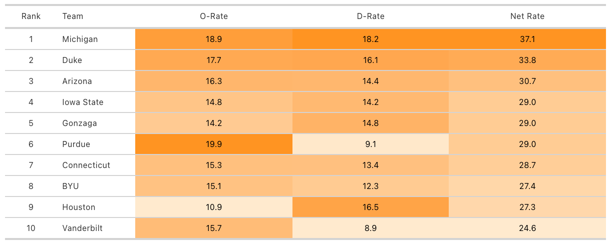
Note that the table could have also been saved as a PDF by changing the file extension in the gtsave( ) function to .pdf instead of .png.
# Save the table as a PDF file.

gtsave(rankings_table, "Miyakawa_Top10_Teams.pdf")