| year | heat_pump | gas_oil |
|---|---|---|
| 2005 | 2136525 | 3623703 |
| 2006 | 2118469 | 3289334 |
| 2007 | 1898905 | 2865658 |
| 2008 | 1865310 | 2338932 |
| 2009 | 1642064 | 2230147 |
| 2010 | 1747920 | 2509724 |
| 2011 | 1765002 | 2264407 |
| 2012 | 1697796 | 2279377 |
| 2013 | 1968632 | 2633904 |
| 2014 | 2353990 | 2769438 |
| 2015 | 2269196 | 2852384 |
| 2016 | 2429867 | 2980287 |
| 2017 | 2619782 | 3171036 |
| 2018 | 2920080 | 2455000 |
| 2019 | 3110888 | 3494006 |
| 2020 | 3418478 | 3387681 |
| 2021 | 3916766 | 4048442 |
| 2022 | 4334479 | 3901383 |
| 2023 | 3616632 | 3012135 |
| 2024 | 4122004 | 3150713 |
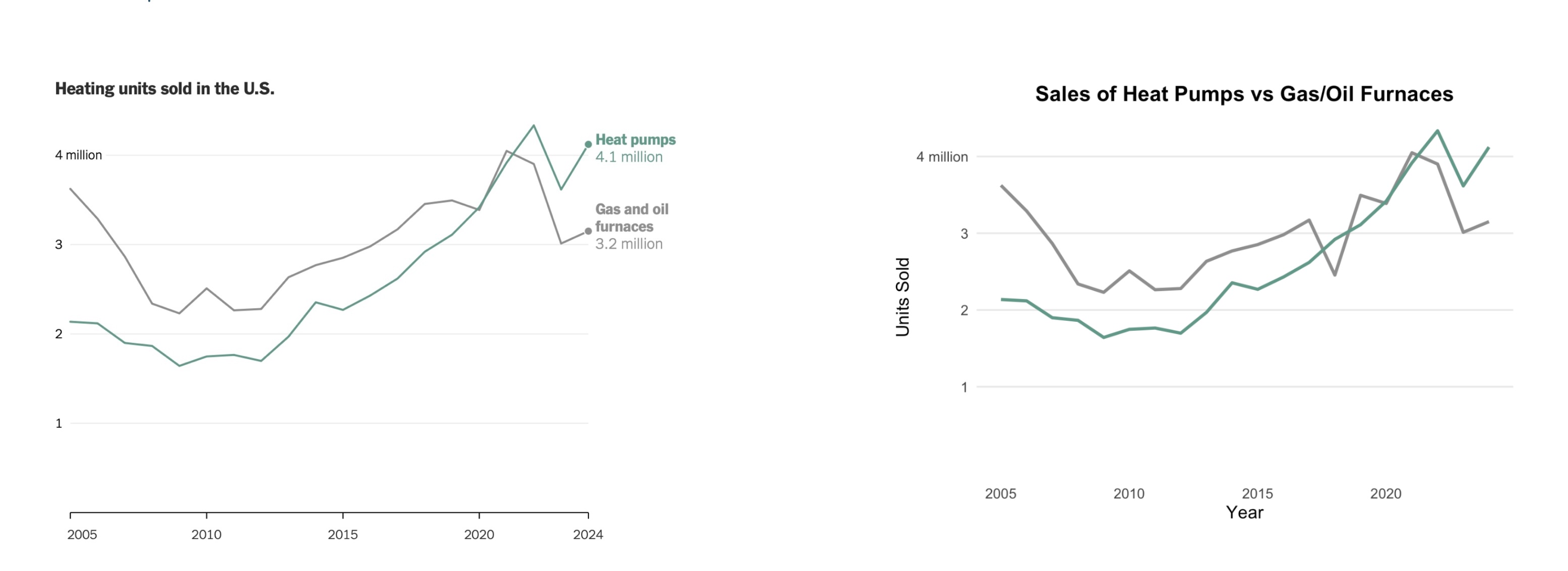
Recreate A New York Times Graphic Challenge
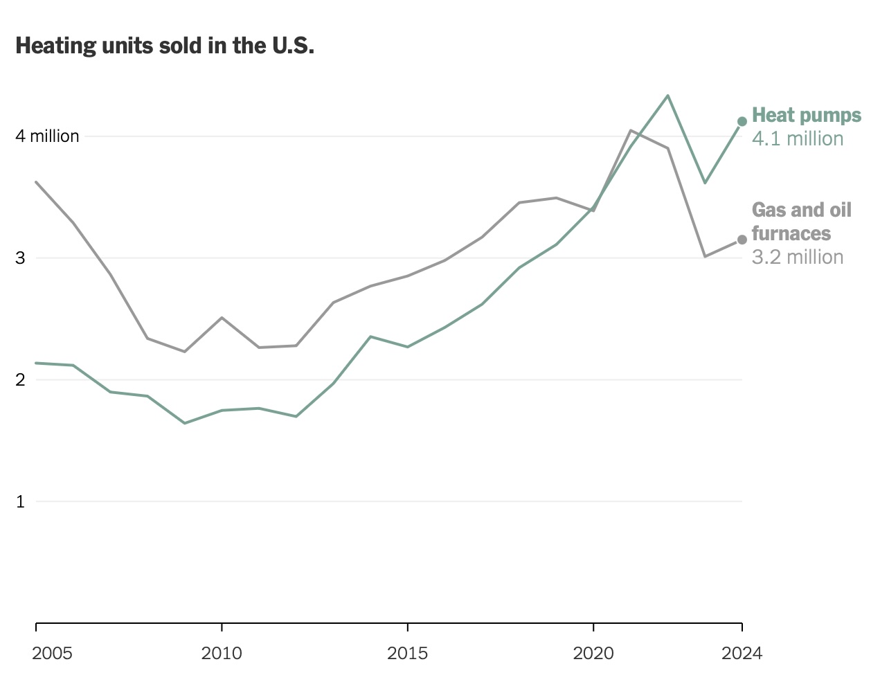
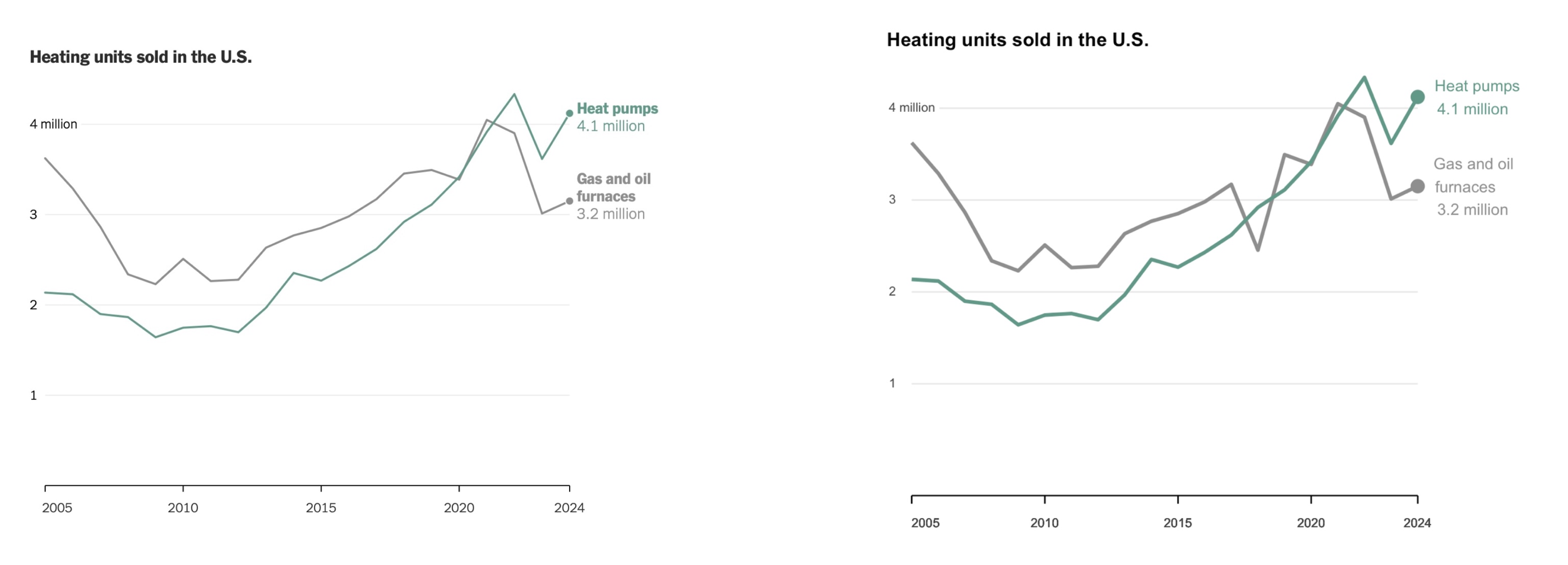
For this exercise, we are going to try to recreate a graphic from a New York Times article. The original graphic can be found from the July 16, 2025 issue of the New York Times.
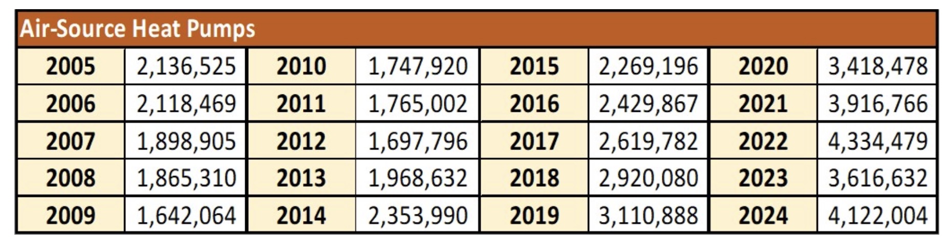
The article discusses the impact of a new policy on the number of heat pumps that are sold versus the number of gas/oil furnaces that are sold. The author uses data from the past twenty years to compare the sales of the two types of heating systems.
You can find the data about heat pumps from THIS source.
You can find the data about gas/oil furnaces from THIS source.

We want to create a line graph that shows the sales of heat pumps and gas/oil furnaces over the past twenty years. The x-axis should be the year, and the y-axis should be the number of units sold. The two lines should be different colors, and there should be a legend that indicates which line is which.
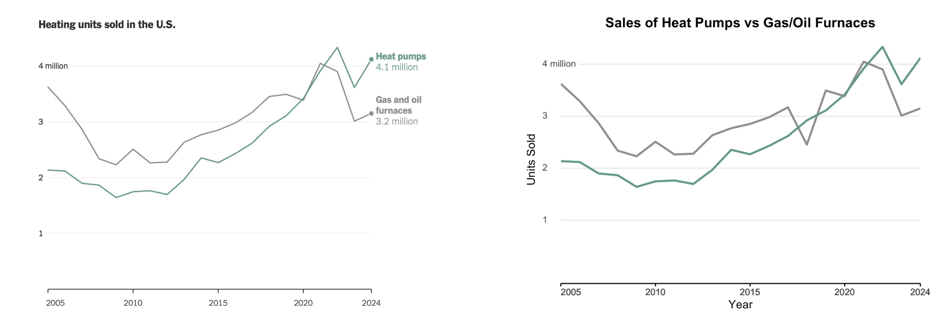
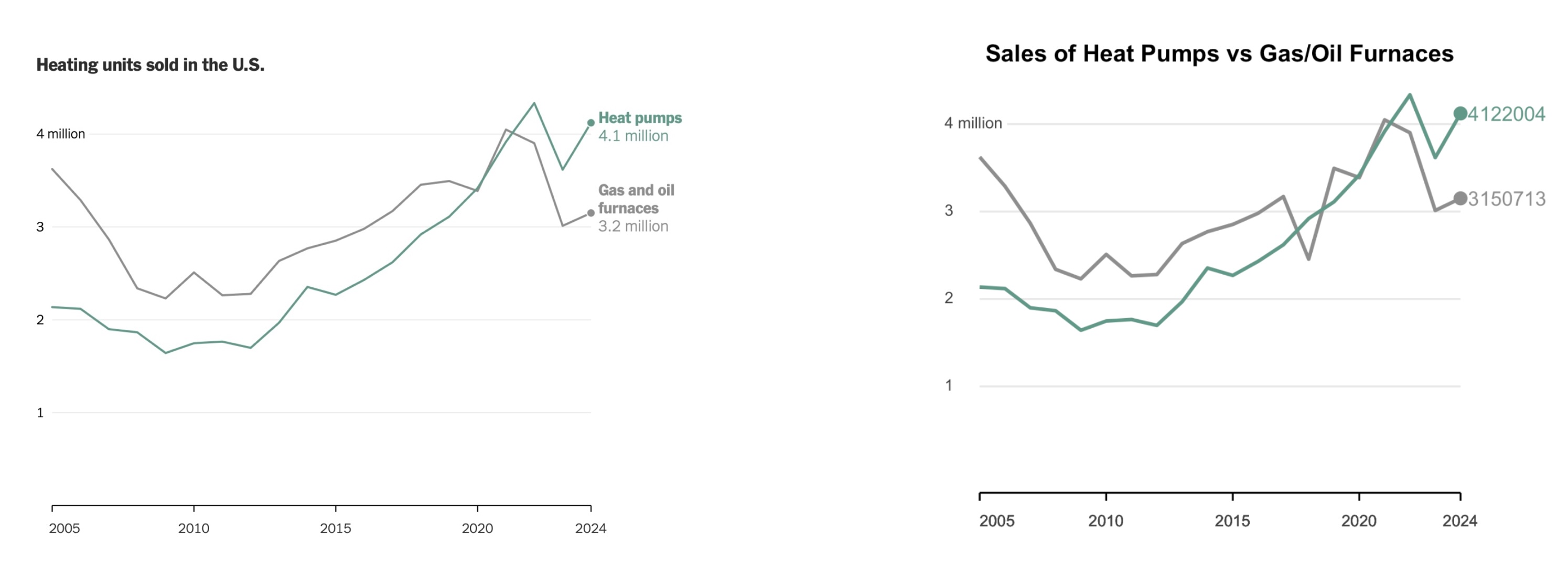
Here is the graphic that was created by the New York Times:
The data has been compiled and saved to a file called NY_Times_sales_data.csv and can be downloaded here :
By now, creating a line graph in R should be a familiar task. However, this exercise is a bit different because we are trying to recreate a specific graphic from the New York Times. It is the small aesthetic details that make the difference in this case, as well as make this more of a challenge.
The first question we want to ask is if this data is tidy? Let’s think about the variables. We ask the following questions :
- What is the year?
- What is the type of heating system (heat pump or gas / oil)?
- How many units were sold?
That means we need a column for each of these variables. We do not have that here.
So the first task we need to do is to clean the data so that it is in the correct format.
We need to make sure that we have a column for the year, a column for the type of heating system, and a column for the number of units sold. Here are the first ten rows.
| year | heating_system | units_sold |
|---|---|---|
| 2005 | heat_pump | 2136525 |
| 2005 | gas_oil | 3623703 |
| 2006 | heat_pump | 2118469 |
| 2006 | gas_oil | 3289334 |
| 2007 | heat_pump | 1898905 |
| 2007 | gas_oil | 2865658 |
| 2008 | heat_pump | 1865310 |
| 2008 | gas_oil | 2338932 |
| 2009 | heat_pump | 1642064 |
| 2009 | gas_oil | 2230147 |
How can we recreate this graphic using R? Let’s think about we will need :
- A line graph, so we will need
geom_line(). - A way to differentiate the two lines, so we will need to use the
coloraesthetic. - We need a point at the end of the line, so
geom_point()will be useful. - A way to customize the graph to match the style of the New York Times graphic, so we will need to use
theme()andtheme_minimal().
We will probably have a few other challenges, but this is a good place to start:
In the aesthetics :
- Make the defualt x values be the year.
- Make the y values be the number of units sold.
- We will differentiate the data by using a different color for the heating system.
ggplot(aes(x = year, y = units_sold, color = heating_system))We can then determine :
- Size of the line
- size of the points
- Color of the lines
geom_line(linewidth = 1.2) +
geom_point(size = 3) +
scale_color_manual(values = c("heat_pump" = "#FF5733", "gas_oil" = "#33C1FF"))
We can then add some :
- labels
- theme information (pick some generic ones to get started)
labs(title = "Sales of Heat Pumps vs Gas/Oil Furnaces",
x = "Year",
y = "Units Sold",
color = "Heating System") +
theme_minimal(base_size = 14) +
theme(
plot.title = element_text(hjust = 0.5, face = "bold"),
legend.position = "bottom"
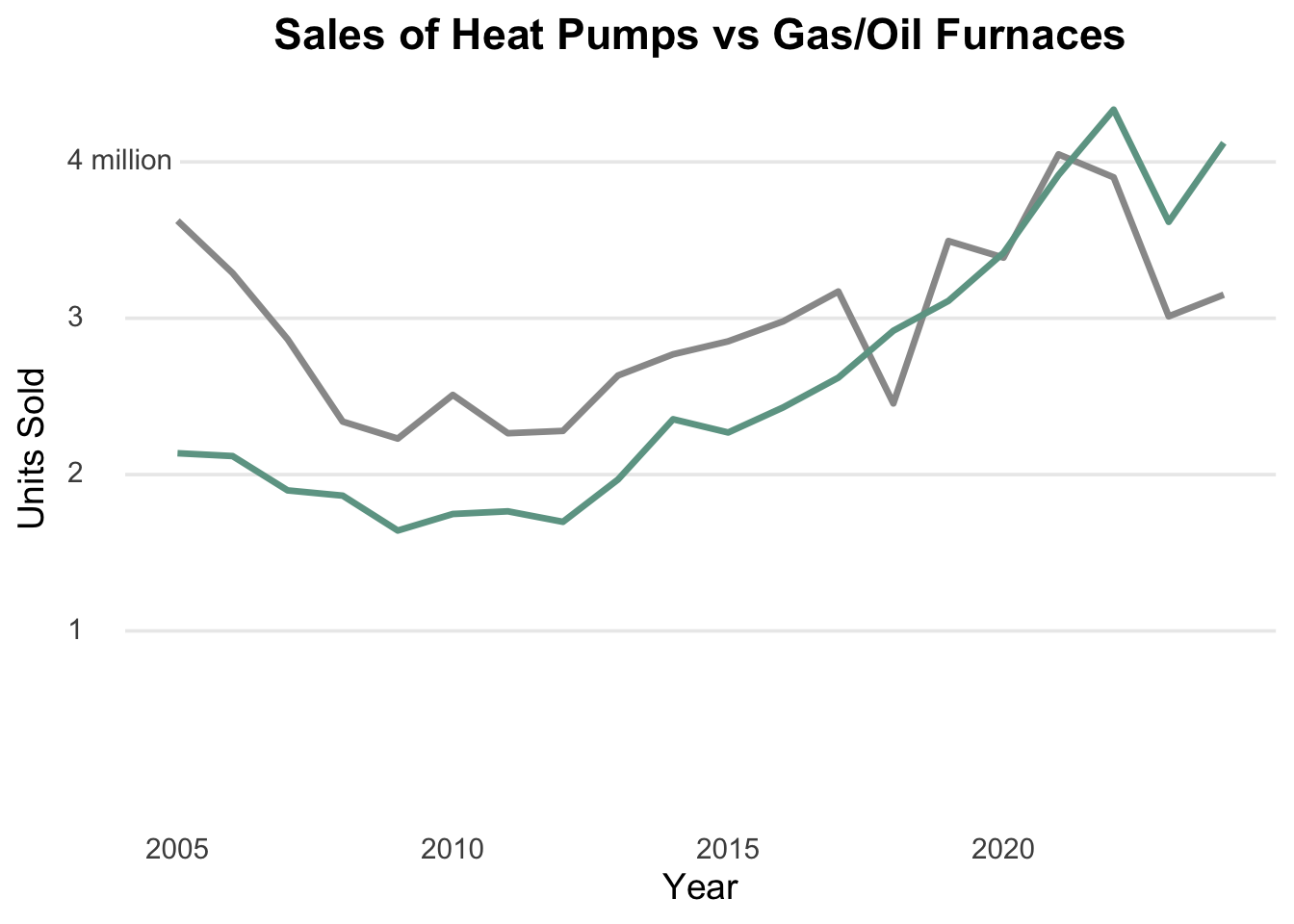
)We will then put it all together to create our first attempt at the graph:
sales_data_tidy |>
  ggplot(aes(x = year, y = units_sold, color = heating_system)) +
  geom_line(linewidth = 1.2) +
  geom_point(size = 3) +
  scale_color_manual(values = c("heat_pump" = "#FF5733", "gas_oil" = "#33C1FF")) +
  labs(title = "Sales of Heat Pumps vs Gas/Oil Furnaces",
       x = "Year",
       y = "Units Sold",
       color = "Heating System") +
  theme_minimal(base_size = 14) +
  theme(
    plot.title = element_text(hjust = 0.5, face = "bold"),
    legend.position = "bottom"
  )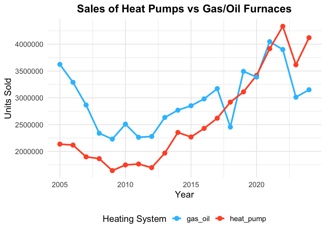
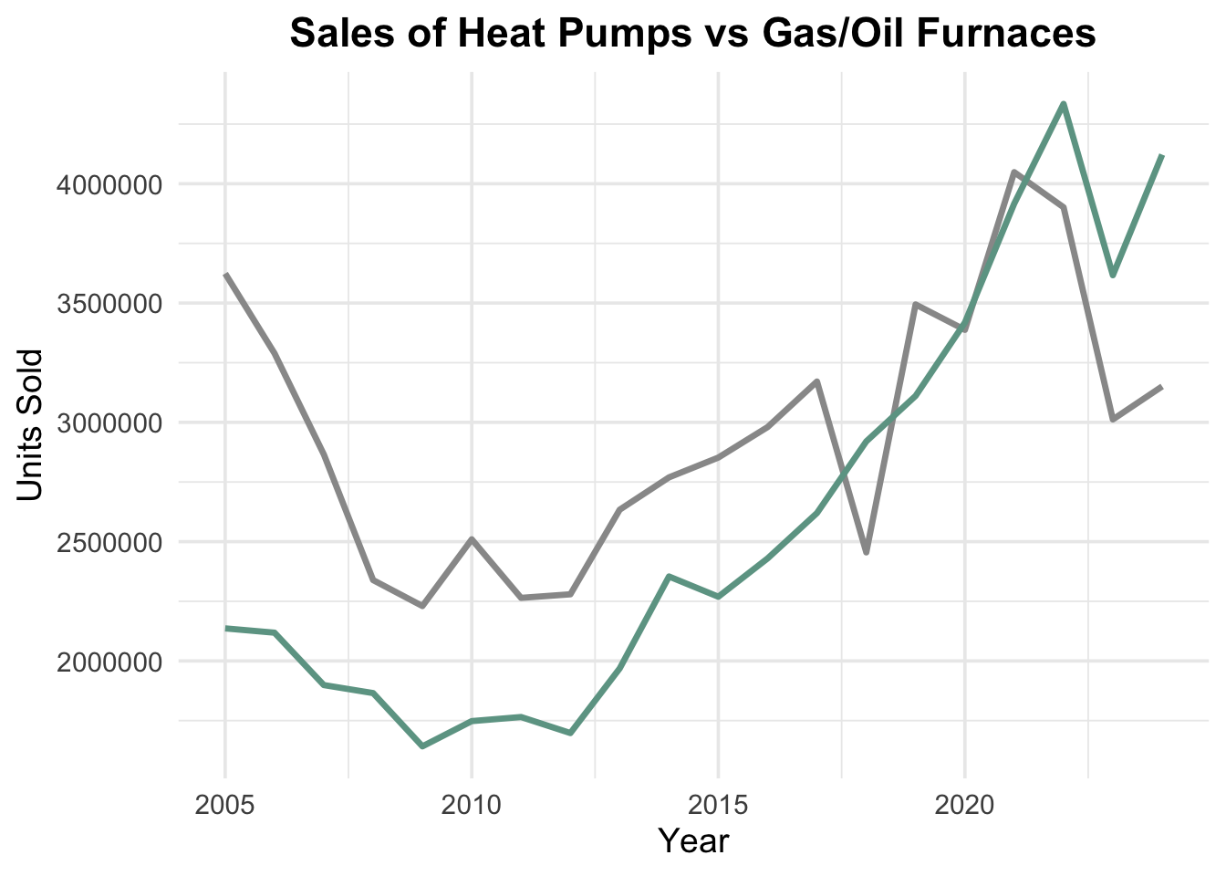
When we compare this first try to the original graphic, we can see that we are close, but there are some differences.
The shape of the graph is good, but there are some steps we still need to do :
- The colors are different.
- We need to remove the points on the lines.
- The legend needs to be removed.
- The grid lines are not quite right. (Major and minor)
- The title is not quite right.
- The y-axis is not formatted correctly.
- The x-axis is not formatted correctly.
- The font is not quite right.
Let’s start with the colors. We can use the scale_color_manual() function to change the colors of the lines. The New York Times uses a specific color palette, so we will use those colors.
There are several ways to get the colors for the heat pump and gas/oil lines.
You can use a color picker tool to get the hex codes for the colors, or you can use a color palette generator to create a palette that matches the New York Times style. You could also look at the HTML code from the webpage to see which colors are chosen.
For this graph, the colors picked are :
- Heat Pump : #6da393
- Gas/Oil : #999
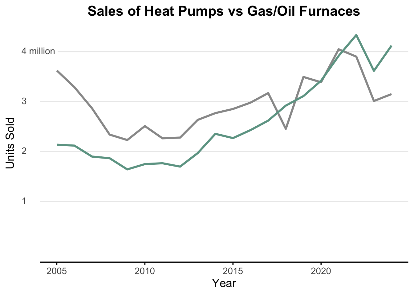
Let’s use these colors in our graph and also do a couple of easy fixes by not using the points on the lines and removing the legend title by changing the position from bottom to none
sales_data_tidy |>
  ggplot(aes(x = year, y = units_sold, color = heating_system)) +
  geom_line(linewidth = 1.2) +
  scale_color_manual(values = c("heat_pump" = "#6da393", "gas_oil" = "#999")) +
  labs(title = "Sales of Heat Pumps vs Gas/Oil Furnaces",
       x = "Year",
       y = "Units Sold",
       color = "Heating System") +
  theme_minimal(base_size = 14) +
  theme(
    plot.title = element_text(hjust = 0.5, face = "bold"),
    legend.position = "none"
  )
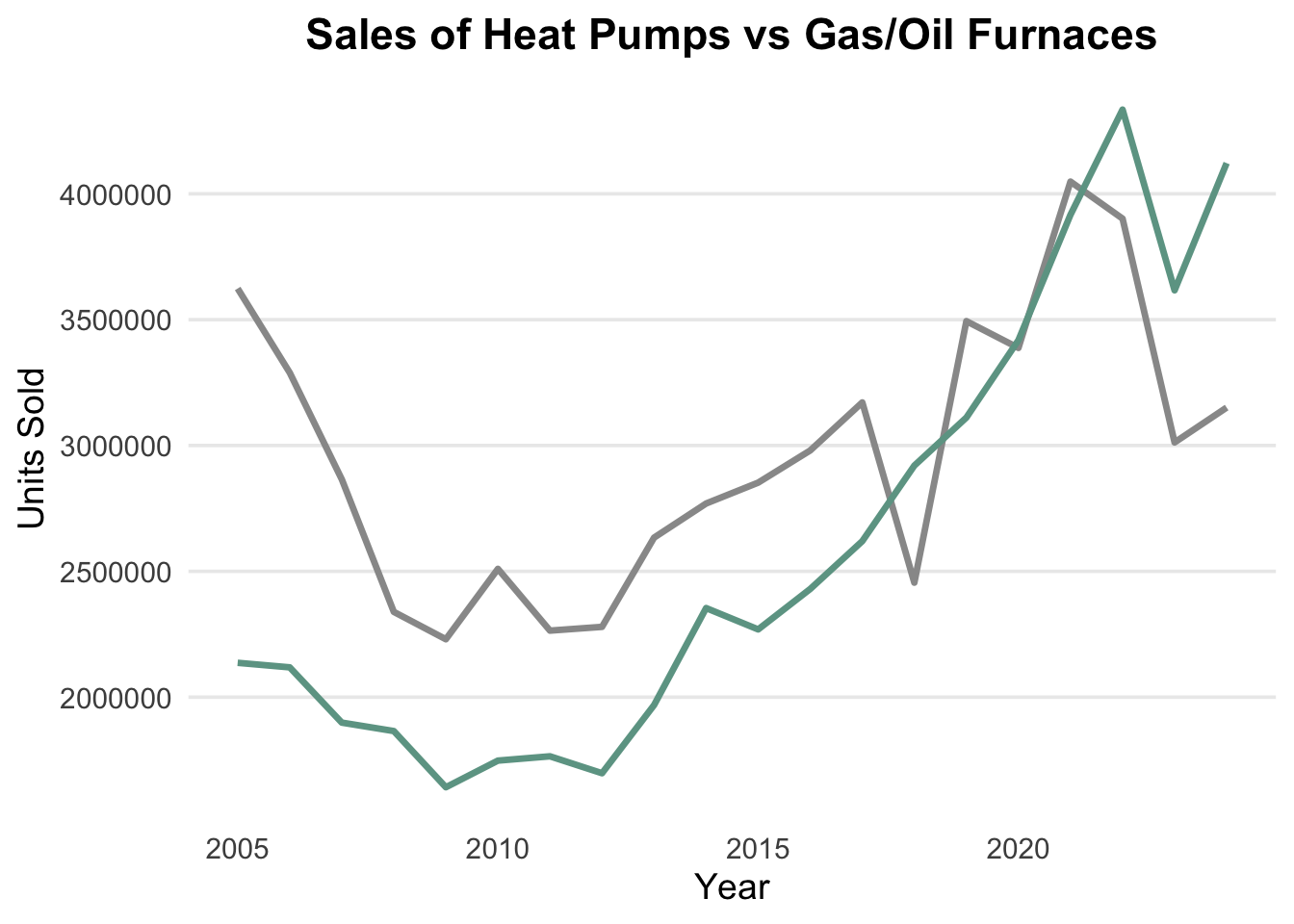
We can now remove the panel grids in the background of the graph by using the panel.grid argument in the theme() function. We will do this in two steps.
When we look at the grid, we can see that there are two types of grid lines :
- Major grid lines that run horizontally across the graph.
- Minor grid lines that run vertically across the graph.
We can remove the minor grid lines by using the panel.grid.minor argument. We do not want to remove the major grid lines for the y axis, so we will leave that as is. We can also remove the major grid lines for the x axis by using the panel.grid.major.x argument.
sales_data_tidy |>
  ggplot(aes(x = year, y = units_sold, color = heating_system)) +
  geom_line(linewidth = 1.2) +
  scale_color_manual(values = c("heat_pump" = "#6da393", "gas_oil" = "#999")) +
  labs(title = "Sales of Heat Pumps vs Gas/Oil Furnaces",
       x = "Year",
       y = "Units Sold",
       color = "Heating System") +
  theme_minimal(base_size = 14) +
  theme(
    plot.title = element_text(hjust = 0.5, face = "bold"),
    legend.position = "none",
    panel.grid.minor = element_blank(),
    panel.grid.major.x = element_blank()
  )
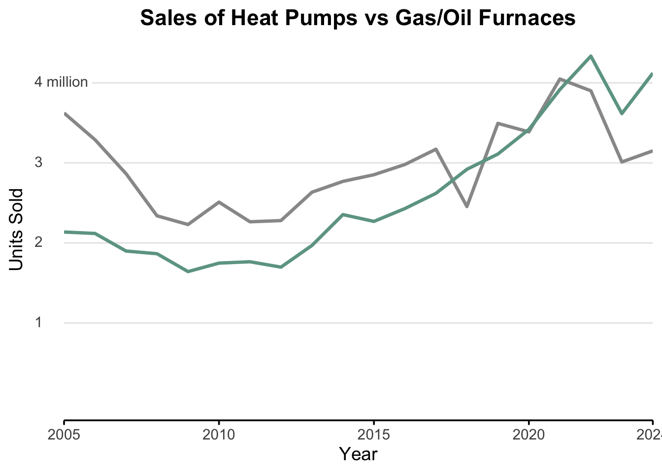
Let’s turn our attention to the y-axis. We want to format the y-axis so that it shows the numbers in a more readable format. We can use the scale_y_continuous() package to do this. We want to :
- Have the numbers go from 1 to 4, instead of 1,000,000 to 4,000,000.
- We don’t want to change the actual values, just the way they are displayed.
- We can use the
breaksargument to set the breaks on the y-axis as 1 million to 4 million
To change the values on the y-axis, we will take advantage of the scale_y_continuous() function. This function allows us to customize the y-axis in a variety of ways, including allowing us to set the breaks to be the values we want.
scale_y_continuous(breaks = c(1,2,3,4) * 1000000)We can now add this to our ggplot() command.
sales_data_tidy |>
  ggplot(aes(x = year, y = units_sold, color = heating_system)) +
  geom_line(linewidth = 1.2) +
  scale_color_manual(values = c("heat_pump" = "#6da393", "gas_oil" = "#999")) +
  scale_y_continuous(breaks = c(1,2,3,4) * 1000000) +
  labs(title = "Sales of Heat Pumps vs Gas/Oil Furnaces",
       x = "Year",
       y = "Units Sold",
       color = "Heating System") +
  theme_minimal(base_size = 14) +
  theme(
    plot.title = element_text(hjust = 0.5, face = "bold"),
    legend.position = "none",
    panel.grid.minor = element_blank(),
    panel.grid.major.x = element_blank()
  )
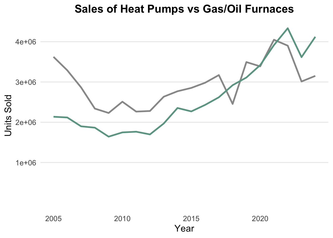
Getting closer!
There are a couple of things we need to clean up before moving to the next idea.
Notice the y-axis doesn’t have the labels that we want and it also doesn’t go down as far as we need.
- We can add limits to the y-axis using the
limitsargument in thescale_y_continuous()function. - I will start the y-axis at 0 and we can manually set it to end wherever we want. I will use
NAto let R determine the upper limit based on the data.
sales_data_tidy |>
  ggplot(aes(x = year, y = units_sold, color = heating_system)) +
  geom_line(linewidth = 1.2) +
  scale_color_manual(values = c("heat_pump" = "#6da393", "gas_oil" = "#999")) +
  scale_y_continuous(breaks = c(1,2,3,4) * 1000000, limits= c(0, NA)) +
  labs(title = "Sales of Heat Pumps vs Gas/Oil Furnaces",
       x = "Year",
       y = "Units Sold",
       color = "Heating System") +
  theme_minimal(base_size = 14) +
  theme(
    plot.title = element_text(hjust = 0.5, face = "bold"),
    legend.position = "none",
    panel.grid.minor = element_blank(),
    panel.grid.major.x = element_blank()
  )
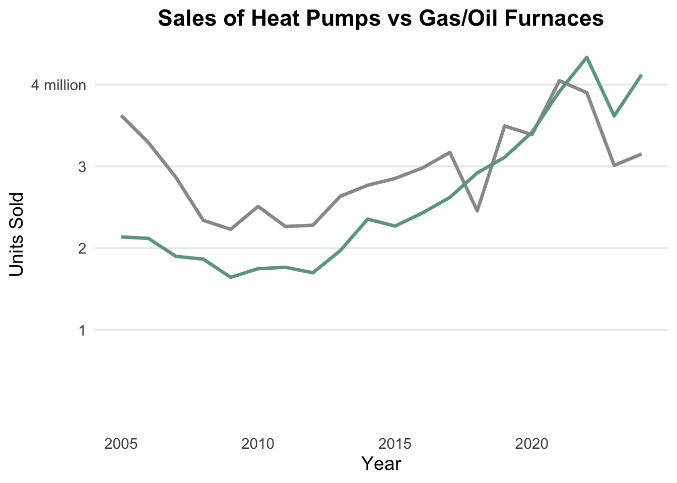
Now that we have the breaks set up, we want to relabel them as simply “1”, “2”, “3”, and “4 million” to match the graphic.
We can use the labels argument in the scale_y_continuous() function to do this.
sales_data_tidy |>
  ggplot(aes(x = year, y = units_sold, color = heating_system)) +
  geom_line(linewidth = 1.2) +
  scale_color_manual(values = c("heat_pump" = "#6da393", "gas_oil" = "#999")) +
  scale_y_continuous(breaks = c(1,2,3,4) * 1000000,
                     limits= c(0, NA),
                     labels = c("1", "2", "3", "4 million")) +
  labs(title = "Sales of Heat Pumps vs Gas/Oil Furnaces",
       x = "Year",
       y = "Units Sold",
       color = "Heating System") +
  theme_minimal(base_size = 14) +
  theme(
    plot.title = element_text(hjust = 0.5, face = "bold"),
    legend.position = "none",
    panel.grid.minor = element_blank(),
    panel.grid.major.x = element_blank()
  )
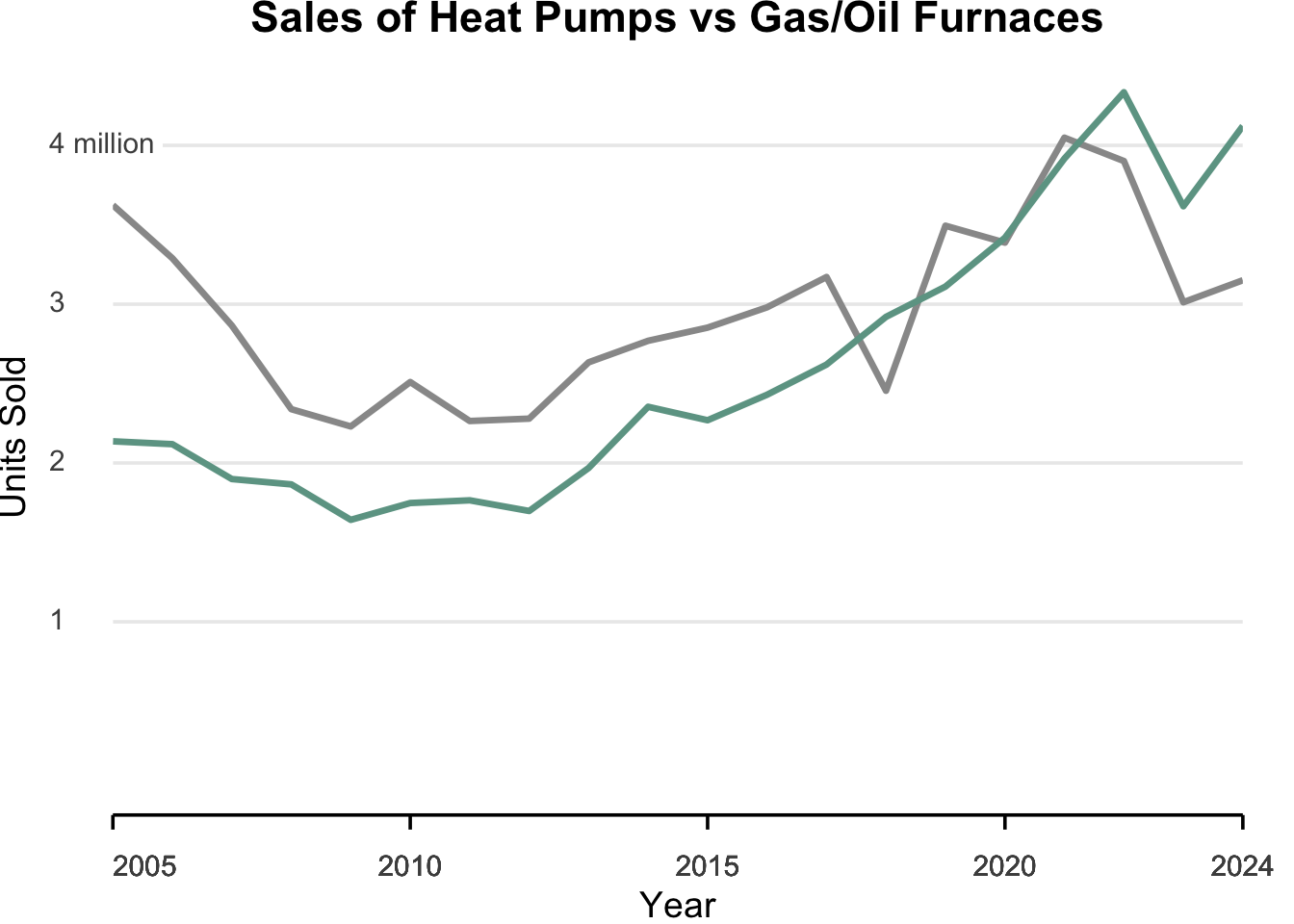
Let’s do a comparison with the original graphic to see where we are :
There is still an issue with the y-axis. If you look closely, you will see the original graphic has the text justified left and ours is justified right. We can fix this by using the axis.text.y argument in the theme() function. We will set the hjust argument to 0 to left justify the text. We will place this in the theme() function.
axis.text.y = element_text(hjust = 0)Here is what the updated graphic looks like after this change:
sales_data_tidy |>
  ggplot(aes(x = year, y = units_sold, color = heating_system)) +
  geom_line(linewidth = 1.2) +
  scale_color_manual(values = c("heat_pump" = "#6da393", "gas_oil" = "#999")) +
  scale_y_continuous(breaks = c(1,2,3,4) * 1000000,
                     limits= c(0, NA),
                     labels = c("1", "2", "3", "4 million")) +
  labs(title = "Sales of Heat Pumps vs Gas/Oil Furnaces",
       x = "Year",
       y = "Units Sold",
       color = "Heating System") +
  theme_minimal(base_size = 14) +
  theme(
    plot.title = element_text(hjust = 0.5, face = "bold"),
    legend.position = "none",
    panel.grid.minor = element_blank(),
    panel.grid.major.x = element_blank(),
    axis.text.y = element_text(hjust = 0)
  )
Almost there! We need to have the horizontal lines reach over the the numbers 1, 2, and 3. We can do this by moving the margins of the graphic. We have to be a little careful because our commands will move all of the lines and if we move them all, the top one will run into the “4 million” text. Here is a plan for doing this.
- Use the
margin()command in thetheme()to move the margins to the left. - We will create a “fill” as a background are all of the text. Since the background is white, we will make the fill white to match.
- We need a little space between the lines and the text, so we will use a
paddin(notice spelling) command to add some space between the lines and the text.
Since all of this is occurring on the y-axis, we will add this to the axis.text.y argument in the theme() function.
Lastly, this is getting away from basic text formatting, so we will change from element_text() to element_markdown() so that we can properly use the markdown commands margin() and padding.
Feel free to play around with the values to see what works best for you. You can also change the color of the padding if you want to see it better. Just make sure you change it back to match the original graphic.
sales_data_tidy |>
  ggplot(aes(x = year, y = units_sold, color = heating_system)) +
  geom_line(linewidth = 1.2) +
  scale_color_manual(values = c("heat_pump" = "#6da393", "gas_oil" = "#999")) +
  scale_y_continuous(breaks = c(1,2,3,4) * 1000000,
                     limits= c(0, NA),
                     labels = c("1", "2", "3", "4 million")) +
  labs(title = "Sales of Heat Pumps vs Gas/Oil Furnaces",
       x = "Year",
       y = "Units Sold",
       color = "Heating System") +
  theme_minimal(base_size = 14) +
  theme(
    plot.title = element_text(hjust = 0.5, face = "bold"),
    legend.position = "none",
    panel.grid.minor = element_blank(),
    panel.grid.major.x = element_blank(),
    axis.text.y = element_markdown(hjust = 0,
                               margin = margin(r = -25),
                               fill="white",
                               paddin = unit(1, "mm"))
  )
We can now start thinking about how to format the x-axis. We will need to add some more information to the theme() function:
- The original graphic has the years formatted as “2005”, “2010”, “2015”, “2020”, and “2024”.
- There is a horizontal line over the years
- There are tick marks over the years, too.
We can add the line to the x-axis using the axis.line.x = element_line() and the ticks using the axis.ticks.x = element_line() arguments in the theme() function.
sales_data_tidy |>
  ggplot(aes(x = year, y = units_sold, color = heating_system)) +
  geom_line(linewidth = 1.2) +
  scale_color_manual(values = c("heat_pump" = "#6da393", "gas_oil" = "#999")) +
  scale_y_continuous(breaks = c(1,2,3,4) * 1000000,
                     limits= c(0, NA),
                     labels = c("1", "2", "3", "4 million")) +
  labs(title = "Sales of Heat Pumps vs Gas/Oil Furnaces",
       x = "Year",
       y = "Units Sold",
       color = "Heating System") +
  theme_minimal(base_size = 14) +
  theme(
    plot.title = element_text(hjust = 0.5, face = "bold"),
    legend.position = "none",
    panel.grid.minor = element_blank(),
    panel.grid.major.x = element_blank(),
    axis.text.y = element_markdown(hjust = 0,
                               margin = margin(r = -25),
                               fill="white",
                               paddin = unit(1, "mm")),
    axis.line.x = element_line(),
    axis.ticks.x = element_line()
  )
We still need to clean this up by adding the breaks to the x-axis so that the years are only shown at the values we want. The original graphic has the years 2005, 2010, 2015, 2020, and 2024. We can use the scale_x_continuous() function to set the breaks on the x-axis to these values.
We can use the scale_x_continuous() function to set the breaks on the x-axis to these values.
scale_x_continuous(breaks = seq(2005, 2024, by = 5))If we add this to our graphic we will get the following:
sales_data_tidy |>
  ggplot(aes(x = year, y = units_sold, color = heating_system)) +
  geom_line(linewidth = 1.2) +
  scale_color_manual(values = c("heat_pump" = "#6da393", "gas_oil" = "#999")) +
  scale_y_continuous(breaks = c(1,2,3,4) * 1000000,
                     limits= c(0, NA),
                     labels = c("1", "2", "3", "4 million")) +
  scale_x_continuous(breaks = seq(2005, 2024, by = 5)) +
  labs(title = "Sales of Heat Pumps vs Gas/Oil Furnaces",
       x = "Year",
       y = "Units Sold",
       color = "Heating System") +
  theme_minimal(base_size = 14) +
  theme(
    plot.title = element_text(hjust = 0.5, face = "bold"),
    legend.position = "none",
    panel.grid.minor = element_blank(),
    panel.grid.major.x = element_blank(),
    axis.text.y = element_markdown(hjust = 0,
                               margin = margin(r = -25),
                               fill="white",
                               paddin = unit(1, "mm")),
    axis.line.x = element_line(),
    axis.ticks.x = element_line()
  )
There is still a little work to do here. Our data only goes to year 2024 and that does not show up on the axis. We will need to adjust the limits of the x-axis by create a vector to hold all the values of the original sequence adding in the last value.
sales_data_tidy |>
  ggplot(aes(x = year, y = units_sold, color = heating_system)) +
  geom_line(linewidth = 1.2) +
  scale_color_manual(values = c("heat_pump" = "#6da393", "gas_oil" = "#999")) +
  scale_y_continuous(breaks = c(1,2,3,4) * 1000000,
                     limits= c(0, NA),
                     labels = c("1", "2", "3", "4 million")) +
  scale_x_continuous(breaks = c(seq(2005, 2020, by = 5), 2024)) +
  labs(title = "Sales of Heat Pumps vs Gas/Oil Furnaces",
       x = "Year",
       y = "Units Sold",
       color = "Heating System") +
  theme_minimal(base_size = 14) +
  theme(
    plot.title = element_text(hjust = 0.5, face = "bold"),
    legend.position = "none",
    panel.grid.minor = element_blank(),
    panel.grid.major.x = element_blank(),
    axis.text.y = element_markdown(hjust = 0,
                               margin = margin(r = -25),
                               fill="white",
                               paddin = unit(1, "mm")),
    axis.line.x = element_line(),
    axis.ticks.x = element_line()
  )
So close!!
Notice the line on the x-axis goes too far in both directions. This is because of some padding that ggplot() automatically adds what is called expansion in the scale_x_continuous() function. There is a small margin added to the left and to the right, so we want to set that expansion to 0 for both.
We can remove this by setting the expand argument to c(0, 0).
scale_x_continuous(breaks = c(seq(2005, 2020, by = 5), 2024), expand = c(0, 0))sales_data_tidy |>
ggplot(aes(x = year, y = units_sold, color = heating_system)) +
geom_line(linewidth = 1.2) +
scale_color_manual(values = c("heat_pump" = "#6da393", "gas_oil" = "#999")) +
scale_y_continuous(breaks = c(1,2,3,4) * 1000000,
limits= c(0, NA),
labels = c("1", "2", "3", "4 million")) +
scale_x_continuous(breaks = c(seq(2005, 2020, by = 5), 2024), expand = c(0,0)) +
labs(title = "Sales of Heat Pumps vs Gas/Oil Furnaces",
x = "Year",
y = "Units Sold",
color = "Heating System") +
theme_minimal(base_size = 14) +
theme(
plot.title = element_text(hjust = 0.5, face = "bold"),
legend.position = "none",
panel.grid.minor = element_blank(),
panel.grid.major.x = element_blank(),
axis.text.y = element_markdown(hjust = 0,
margin = margin(r = -25),
fill="white",
paddin = unit(1, "mm")),
axis.line.x = element_line(),
axis.ticks.x = element_line()
)
If we look closely, there is still some work to do on the x-axis.
- All of the tick marks are centered on the years, except 2005 where it is right justified.
- The last year, 2024, is cut off a bit, so we need to extend the right margin by a little bit.
We can fix the first issue by using the hjust argument in the axis.text.x argument in the theme() function. We will set the hjust to 0.5 to center the text on the tick marks and 0 to left justify the text on the tick marks. If we wanted to right justify the text on the tick marks, we would set the hjust to 1.
So we have 5 values on the x-axis to justify :
axis.text.x = element_text(hjust = c(0, 0.5, 0.5, 0.5, 0.5))To add to the right margin on the x-axis, we use the plot.margin argument in the theme() function.
plot.margin = margin(r=20)We can play around with these values to see what works best for us.
sales_data_tidy |>
  ggplot(aes(x = year, y = units_sold, color = heating_system)) +
  geom_line(linewidth = 1.2) +
  scale_color_manual(values = c("heat_pump" = "#6da393", "gas_oil" = "#999")) +
  scale_y_continuous(breaks = c(1,2,3,4) * 1000000,
                     limits= c(0, NA),
                     labels = c("1", "2", "3", "4 million")) +
  scale_x_continuous(breaks = c(seq(2005, 2020, by = 5), 2024), expand = c(0,0)) +
  labs(title = "Sales of Heat Pumps vs Gas/Oil Furnaces",
       x = "Year",
       y = "Units Sold",
       color = "Heating System") +
  theme_minimal(base_size = 14) +
  theme(
    plot.title = element_text(hjust = 0.5, face = "bold"),
    legend.position = "none",
    panel.grid.minor = element_blank(),
    panel.grid.major.x = element_blank(),
    axis.text.y = element_markdown(hjust = 0,
                               margin = margin(r = -25),
                               fill="white",
                               paddin = unit(1, "mm")),
    axis.line.x = element_line(),
    axis.ticks.x = element_line(),
    axis.text.x = element_text(hjust = c(0, 0.5, 0.5, 0.5, 0.5)),
    plot.margin = margin(r=20)
  )
Warning: Vectorized input to `element_text()` is not officially supported.
ℹ Results may be unexpected or may change in future versions of ggplot2.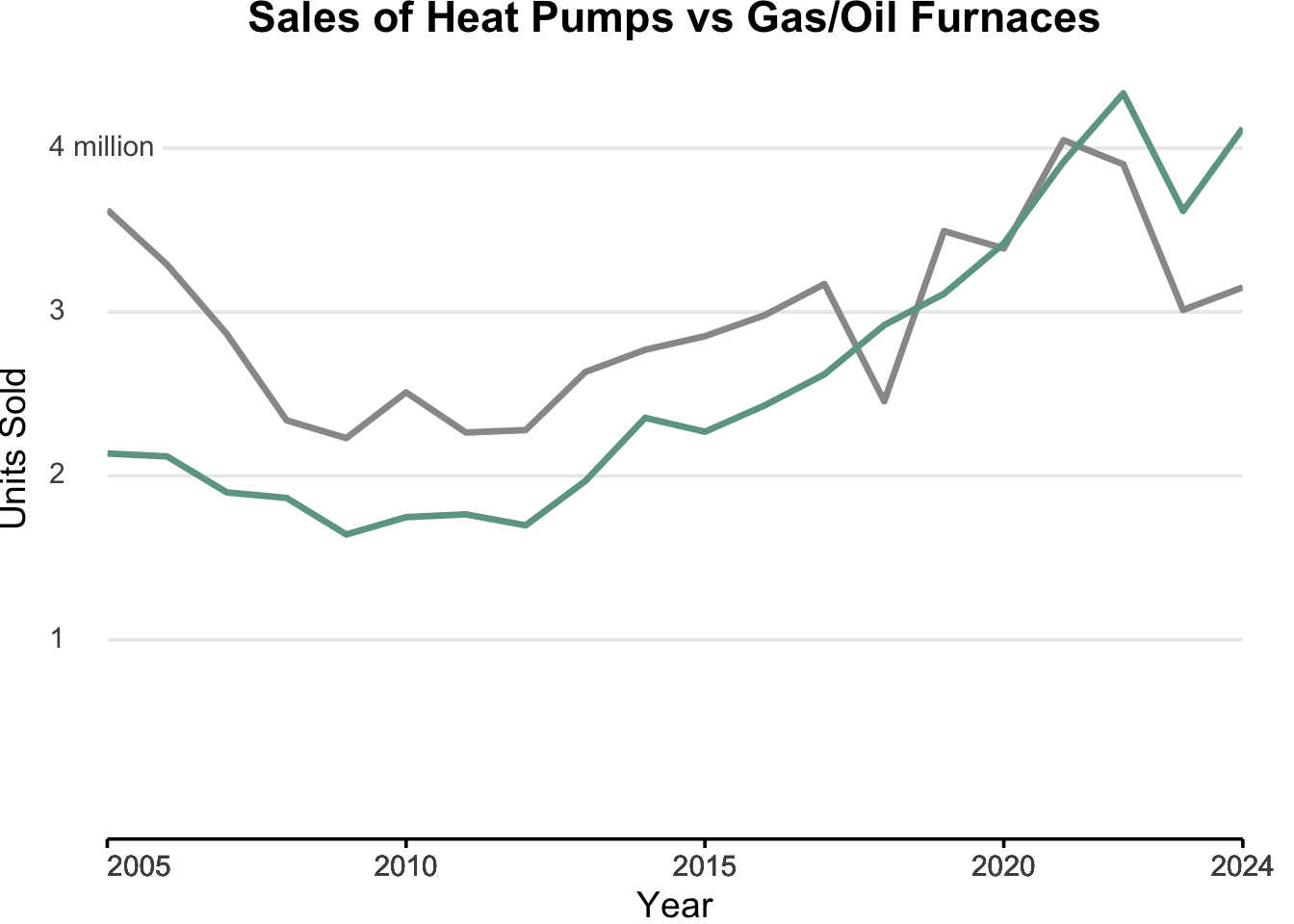
Let’s see how close we are :
The x-axis is almost there. We need to add a little padding between the x-axis and the numbers. In other words, move the x-axis down a little bit. We can add a margin to the axis.text.x argument in the theme() function.
axis.text.x = element_text(hjust = c(0, 0.5, 0.5, 0.5, 0.5),
                           margin = margin(t = 10))
We can also make the tick marks a little longer. We can do this by using the axis.ticks.length argument in the theme() function.
axis.ticks.length = unit(2, "mm")This gives us the following:
sales_data_tidy |>
  ggplot(aes(x = year, y = units_sold, color = heating_system)) +
  geom_line(linewidth = 1.2) +
  scale_color_manual(values = c("heat_pump" = "#6da393", "gas_oil" = "#999")) +
  scale_y_continuous(breaks = c(1,2,3,4) * 1000000,
                     limits= c(0, NA),
                     labels = c("1", "2", "3", "4 million")) +
  scale_x_continuous(breaks = c(seq(2005, 2020, by = 5), 2024), expand = c(0,0)) +
  labs(title = "Sales of Heat Pumps vs Gas/Oil Furnaces",
       x = "Year",
       y = "Units Sold",
       color = "Heating System") +
  theme_minimal(base_size = 14) +
  theme(
    plot.title = element_text(hjust = 0.5, face = "bold"),
    legend.position = "none",
    panel.grid.minor = element_blank(),
    panel.grid.major.x = element_blank(),
    axis.text.y = element_markdown(hjust = 0,
                               margin = margin(r = -25),
                               fill="white",
                               paddin = unit(1, "mm")),
    axis.line.x = element_line(),
    axis.ticks.x = element_line(),
    axis.ticks.length = unit(2, "mm"),
    axis.text.x = element_text(hjust = c(0, 0.5, 0.5, 0.5, 0.5),
                           margin = margin(t = 10)),
    plot.margin = margin(r=20)
  )
Boom. We are now ready to work with the labels.
The first thing you can see is that we are going to need to add some padding to the right of the graph to fit in some text. We. can do this by just increasing what we did before. We can increase the right margin to 120 pixels.
plot.margin = margin(r=120)The original graphic does not have the labels on the x and y axis, so let’s go ahead and remove those by setting the x and y arguments in the labs() function to "".
labs(title = "Sales of Heat Pumps vs Gas/Oil Furnaces",
       x = "",
       y = "",
       color = "Heating System")
sales_data_tidy |>
ggplot(aes(x = year, y = units_sold, color = heating_system)) +
geom_line(linewidth = 1.2) +
scale_color_manual(values = c("heat_pump" = "#6da393", "gas_oil" = "#999")) +
scale_y_continuous(breaks = c(1,2,3,4) * 1000000,
limits= c(0, NA),
labels = c("1", "2", "3", "4 million")) +
scale_x_continuous(breaks = c(seq(2005, 2020, by = 5), 2024), expand = c(0,0)) +
labs(title = "Sales of Heat Pumps vs Gas/Oil Furnaces",
x = "",
y = "",
color = "Heating System") +
theme_minimal(base_size = 14) +
theme(
plot.title = element_text(hjust = 0.5, face = "bold"),
legend.position = "none",
panel.grid.minor = element_blank(),
panel.grid.major.x = element_blank(),
axis.text.y = element_markdown(hjust = 0,
margin = margin(r = -25),
fill="white",
paddin = unit(1, "mm")),
axis.line.x = element_line(),
axis.ticks.x = element_line(),
axis.ticks.length = unit(2, "mm"),
axis.text.x = element_text(hjust = c(0, 0.5, 0.5, 0.5, 0.5),
margin = margin(t = 10)),
plot.margin = margin(r=120)
)
It looks like there are three tasks left to do.
- Add a point to the end of the lines
- Add text at the end of the lines
- Add the appropriate title.
We can add a point to the end of the lines by using the geom_point() function. If we just add the basic geom_point() function, it will add a point to every data point in the graph. We only want to add a point to the end of the lines, so we will need to filter the data to only include the last year for each heating system. We can do this by using the filter() function from the dplyr package. We will filter the data to only include the last year for each heating system.
library(dplyr)
sales_data_last <- sales_data_tidy %>%
  filter(year == 2024)
When we call geom_point() we will use the data argument to specify that we want to use the sales_data_last data frame.
geom_point(data = sales_data_last, size = 4)Here is our latest attempt:
sales_data_last <- sales_data_tidy %>%
  filter(year == 2024)

sales_data_tidy |>
  ggplot(aes(x = year, y = units_sold, color = heating_system)) +
  geom_line(linewidth = 1.2) +
  geom_point(data = sales_data_last, size = 4) +
  scale_color_manual(values = c("heat_pump" = "#6da393", "gas_oil" = "#999")) +
  scale_y_continuous(breaks = c(1,2,3,4) * 1000000,
                     limits= c(0, NA),
                     labels = c("1", "2", "3", "4 million")) +
  scale_x_continuous(breaks = c(seq(2005, 2020, by = 5), 2024), expand = c(0,0)) +
  labs(title = "Sales of Heat Pumps vs Gas/Oil Furnaces",
       x = "",
       y = "",
       color = "Heating System") +
  theme_minimal(base_size = 14) +
  theme(
    plot.title = element_text(hjust = 0.5, face = "bold"),
    legend.position = "none",
    panel.grid.minor = element_blank(),
    panel.grid.major.x = element_blank(),
    axis.text.y = element_markdown(hjust = 0,
                               margin = margin(r = -25),
                               fill="white",
                               paddin = unit(1, "mm")),
    axis.line.x = element_line(),
    axis.ticks.x = element_line(),
    axis.ticks.length = unit(2, "mm"),
    axis.text.x = element_text(hjust = c(0, 0.5, 0.5, 0.5, 0.5),
                           margin = margin(t = 10)),
    plot.margin = margin(r=120)
  )
If you notice, the point got cut off a bit. This is, again, because of the defaults on `ggplot(). We can fix this by adding the coord_cartesian() function to the graph. We can use the clip = "off" argument to allow the point to be drawn outside the plot area. We will add this just before we start the theme().
sales_data_last <- sales_data_tidy %>%
  filter(year == 2024)

sales_data_tidy |>
  ggplot(aes(x = year, y = units_sold, color = heating_system)) +
  geom_line(linewidth = 1.2) +
  geom_point(data = sales_data_last, size = 4) +
  scale_color_manual(values = c("heat_pump" = "#6da393", "gas_oil" = "#999")) +
  scale_y_continuous(breaks = c(1,2,3,4) * 1000000,
                     limits= c(0, NA),
                     labels = c("1", "2", "3", "4 million")) +
  scale_x_continuous(breaks = c(seq(2005, 2020, by = 5), 2024), expand = c(0,0)) +
  labs(title = "Sales of Heat Pumps vs Gas/Oil Furnaces",
       x = "",
       y = "",
       color = "Heating System") +
  coord_cartesian(clip = "off") +
  theme_minimal(base_size = 14) +
  theme(
    plot.title = element_text(hjust = 0.5, face = "bold"),
    legend.position = "none",
    panel.grid.minor = element_blank(),
    panel.grid.major.x = element_blank(),
    axis.text.y = element_markdown(hjust = 0,
                               margin = margin(r = -25),
                               fill="white",
                               paddin = unit(1, "mm")),
    axis.line.x = element_line(),
    axis.ticks.x = element_line(),
    axis.ticks.length = unit(2, "mm"),
    axis.text.x = element_text(hjust = c(0, 0.5, 0.5, 0.5, 0.5),
                           margin = margin(t = 10)),
    plot.margin = margin(r=120)
  )
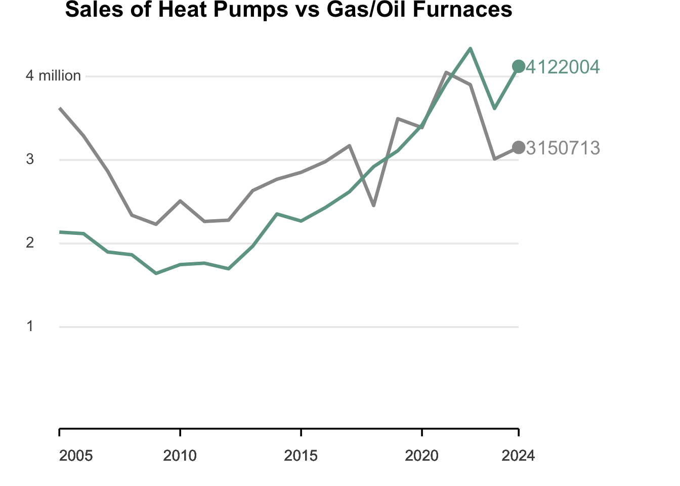
We now want to add text to go along with the last point. We will be using the geom_text() function to add the text, but we have to be careful. The default will add text to all the points and we just want text at the last point. We will use the data argument to specify that we want to use only the sales_data_last data frame. We will then use the label argument to specify the text we want to add.
We could add something like this :
  geom_text(data = sales_data_last,
            aes(label = units_sold),
            hjust = -0.1,
            size = 5)
This will add text to the last points and the text we are using in this case is the units sold (heat - 4122004. and gas/oil - 3150713). We are adjusting the hjust argument to -0.1 to move the text a little to the left closer to the point and the size argument to 5 to make the text a little larger. We can play with these when we get done to see what looks the best for this problem.
sales_data_last <- sales_data_tidy %>%
filter(year == 2024)
sales_data_tidy |>
ggplot(aes(x = year, y = units_sold, color = heating_system)) +
geom_line(linewidth = 1.2) +
geom_point(data = sales_data_last, size = 4) +
geom_text(data = sales_data_last,
aes(label = units_sold),
hjust = -0.1,
size = 5) +
scale_color_manual(values = c("heat_pump" = "#6da393", "gas_oil" = "#999")) +
scale_y_continuous(breaks = c(1,2,3,4) * 1000000,
limits= c(0, NA),
labels = c("1", "2", "3", "4 million")) +
scale_x_continuous(breaks = c(seq(2005, 2020, by = 5), 2024), expand = c(0,0)) +
labs(title = "Sales of Heat Pumps vs Gas/Oil Furnaces",
x = "",
y = "",
color = "Heating System") +
coord_cartesian(clip = "off") +
theme_minimal(base_size = 14) +
theme(
plot.title = element_text(hjust = 0.5, face = "bold"),
legend.position = "none",
panel.grid.minor = element_blank(),
panel.grid.major.x = element_blank(),
axis.text.y = element_markdown(hjust = 0,
margin = margin(r = -25),
fill="white",
paddin = unit(1, "mm")),
axis.line.x = element_line(),
axis.ticks.x = element_line(),
axis.ticks.length = unit(2, "mm"),
axis.text.x = element_text(hjust = c(0, 0.5, 0.5, 0.5, 0.5),
margin = margin(t = 10)),
plot.margin = margin(r=120)
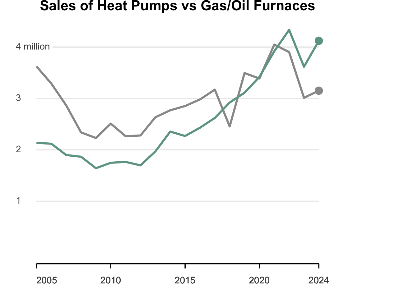
)
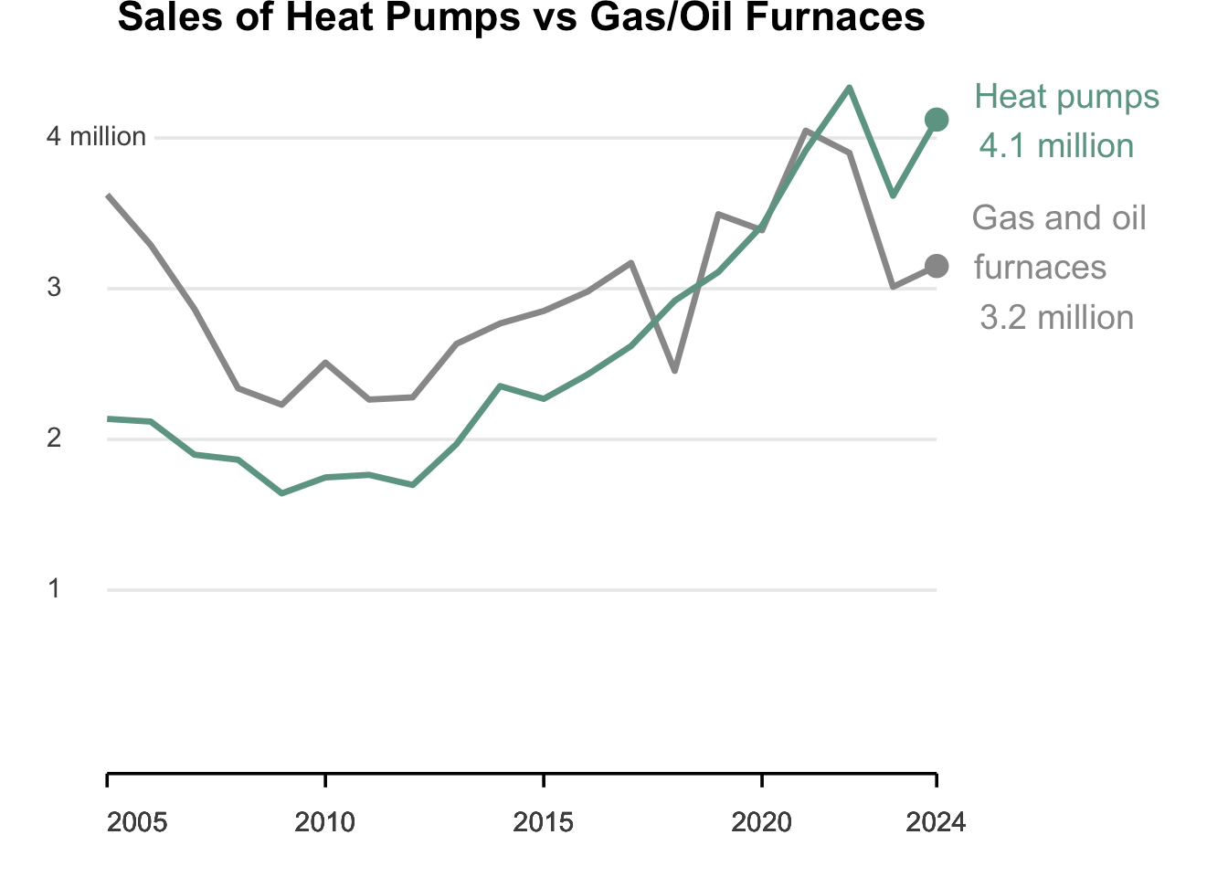
Let’s check to see how close we are to the original graphic.
We now want to format the text next to the points. We can add a label() in the aes() portion of geom_text() to specify the text we want to add.
We will want to use some markdown notation to format the text. We will use the \n tag to add a line break.
  geom_text(data = sales_data_last,
            aes(label = c("Heat pumps\n 4.1 million",
                          "Gas and oil\n furnaces\n 3.2 million")),
            hjust = -0.2,
            size = 5
Note that I adjusted the hjust to -0.2 to move the text a little more to the right.
sales_data_last <- sales_data_tidy %>%
  filter(year == 2024)

sales_data_tidy |>
  ggplot(aes(x = year, y = units_sold, color = heating_system)) +
  geom_line(linewidth = 1.2) +
  geom_point(data = sales_data_last, size = 4) +
  geom_text(data = sales_data_last,
            aes(label = c("Heat pumps\n 4.1 million",
                          "Gas and oil\n furnaces\n 3.2 million")),
            hjust = -0.2,
            size = 5) +
  scale_color_manual(values = c("heat_pump" = "#6da393", "gas_oil" = "#999")) +
  scale_y_continuous(breaks = c(1,2,3,4) * 1000000,
                     limits= c(0, NA),
                     labels = c("1", "2", "3", "4 million")) +
  scale_x_continuous(breaks = c(seq(2005, 2020, by = 5), 2024), expand = c(0,0)) +
  labs(title = "Sales of Heat Pumps vs Gas/Oil Furnaces",
       x = "",
       y = "",
       color = "Heating System") +
  coord_cartesian(clip = "off") +
  theme_minimal(base_size = 14) +
  theme(
    plot.title = element_text(hjust = 0.5, face = "bold"),
    legend.position = "none",
    panel.grid.minor = element_blank(),
    panel.grid.major.x = element_blank(),
    axis.text.y = element_markdown(hjust = 0,
                               margin = margin(r = -25),
                               fill="white",
                               paddin = unit(1, "mm")),
    axis.line.x = element_line(),
    axis.ticks.x = element_line(),
    axis.ticks.length = unit(2, "mm"),
    axis.text.x = element_text(hjust = c(0, 0.5, 0.5, 0.5, 0.5),
                           margin = margin(t = 10)),
    plot.margin = margin(r=120)
  )
There is one item we will not replicate here and that is making some of the text bold. It is certainly possible as you could string together a few pieces of text where one is in bold and the next is not. I will not do that here.
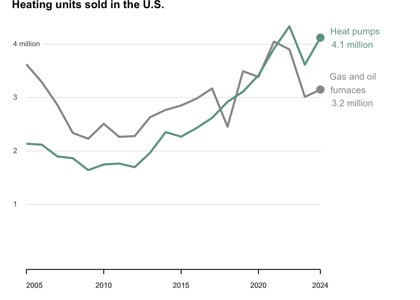
That does bring us to the last item to fix and that is the title.
- It needs to say “Heating units sold in the U.S.
- It needs to be on the left lined up with the plot
- It needs to be bold
labs(title = "Heating units sold in the U.S.",
       x = "",
       y = "",
       color = "Heating System")
I also noticed the size of the text was too large, so I removed the base_size argument from the theme_minimal() function and removed the size = 5 argument from the geom_text() function.
The title many need to be adjusted horizontally, so we may need to add the hjust argument to the plot.title argument in the theme() function. I played around and found -0.1 a good value, but you can see where you want it to be.
Here is where we are now:
sales_data_last <- sales_data_tidy %>%
  filter(year == 2024)

sales_data_tidy |>
  ggplot(aes(x = year, y = units_sold, color = heating_system)) +
  geom_line(linewidth = 1.2) +
  geom_point(data = sales_data_last, size = 4) +
  geom_text(data = sales_data_last,
            aes(label = c("Heat pumps\n 4.1 million",
                          "Gas and oil\n furnaces\n 3.2 million")),
            hjust = -0.2
            ) +
  scale_color_manual(values = c("heat_pump" = "#6da393", "gas_oil" = "#999")) +
  scale_y_continuous(breaks = c(1,2,3,4) * 1000000,
                     limits= c(0, NA),
                     labels = c("1", "2", "3", "4 million")) +
  scale_x_continuous(breaks = c(seq(2005, 2020, by = 5), 2024), expand = c(0,0)) +
  labs(title = "Heating units sold in the U.S.",
       x = "",
       y = "",
       color = "Heating System") +
  coord_cartesian(clip = "off") +
  theme_minimal() +
  theme(
    plot.title = element_text(hjust = -0.1, face = "bold"),
    legend.position = "none",
    panel.grid.minor = element_blank(),
    panel.grid.major.x = element_blank(),
    axis.text.y = element_markdown(hjust = 0,
                               margin = margin(r = -25),
                               fill="white",
                               paddin = unit(1, "mm")),
    axis.line.x = element_line(),
    axis.ticks.x = element_line(),
    axis.ticks.length = unit(2, "mm"),
    axis.text.x = element_text(hjust = c(0, 0.5, 0.5, 0.5, 0.5),
                           margin = margin(t = 10)),
    plot.margin = margin(r=120)
  )
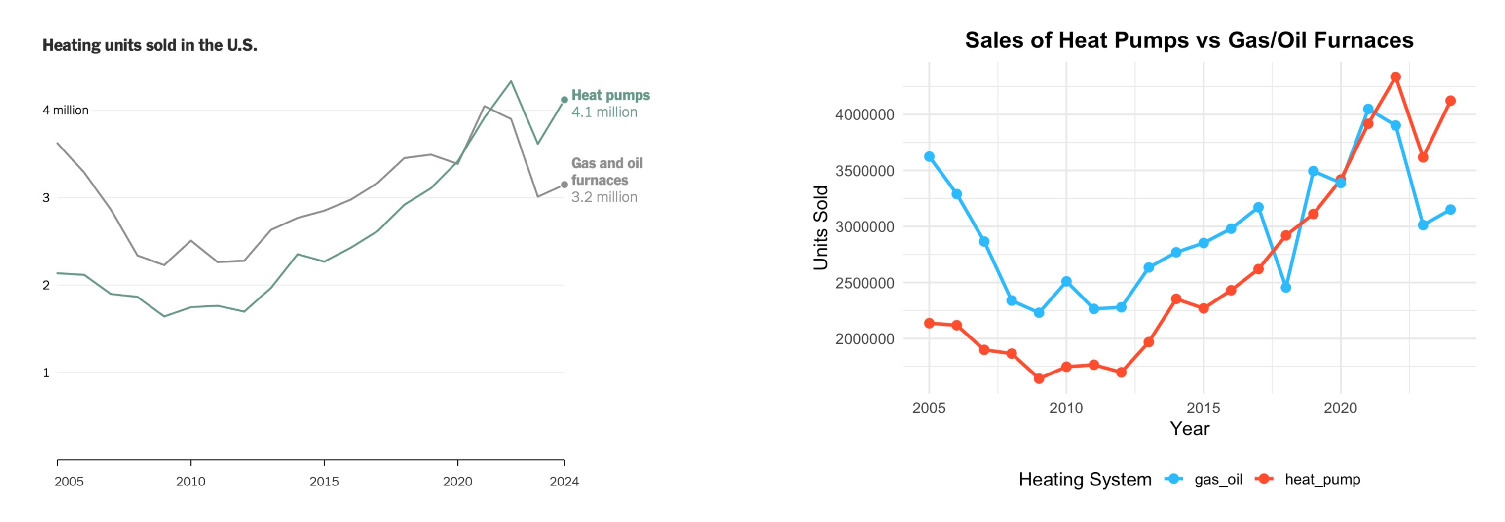
Let’s do one final comparison of images :
There are some small aesthetic differences, but overall we have a very close replica of the original graphic!
Thanks to Spencer Schien for the original challenge and walkthrough at https://www.youtube.com/watch?v=XihJUrDXq6s